Polynomial functions on Young diagrams arising from bipartite graphs

<strong>Polynomial</strong> <strong>functions</strong> on Young diagrams 265
t
z 1 z 2 z 3 z 4 z 5
z
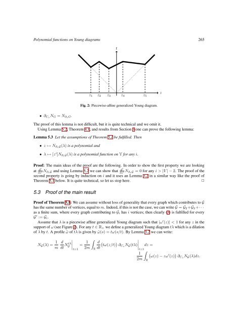
Fig. 2: Piecewise-affine generalized Young diagram.
• ∂ Cz N G = N ∂zG.
The proof of this lemma is not difficult, but it is quite technical and we omit it.
Using Lemma 5.2, Theorem 4.1, and results from Section 3 one can prove the following lemma:
Lemma 5.3 Let the assumptions of Theorem 5.1 be fulfilled. Then
• z ↦→ N ∂zG(λ) is a polynomial and
• λ ↦→ [z i ]N ∂zG(λ) is a polynomial function on Y for any i.
Proof: The main ideas of the proof are the following. In order to show the first property we are looking
d
at i
d
dz
N i ∂zG and using Lemma 5.2 we can show that i
dz
N i ∂zG = 0 for any i > |V | − 2. The proof of the
second property is going by induction on i and it uses an Lemma 3.2 in a similar way like the proof of
Theorem 5.1 below. It is quite technical, so let us stop here.
✷
5.3 Proof of the main result
Proof of Theorem 5.1: We can assume without loss of generality that every graph which contributes to G
has the same number of vertices, equal to m. Indeed, if this is not the case, we can write G = G 2 +G 3 +· · ·
as a finite sum, where every graph contributing to G i has i vertices; then clearly (3) is fulfilled for every
G ′ := G i .
Assume that λ is a piecewise affine generalized Young diagram such that |ω ′ (z)| < 1 for any z in the
support of ω (see Figure 2). For any t ∈ R + we define a generalized Young diagram tλ which is a dilation
of λ by t. A profile ˜ω of tλ is given by ˜ω(s) = tω(s/t). By Lemma 3.2 we can write:
N G (λ) = 1 m
d
dt N G
tλ
∣ = 1 ∫
t=1
2m
R
d ( ) tω(z/t) ∂Cz N G (tλ)
dt
∣ dz =
t=1
∫
1 (
ω(z) − zω ′ (z) ) ∂ Cz N G (λ)dz.
2m
R