Heuristic Methods for Graph Coloring Problems
Heuristic Methods for Graph Coloring Problems
Heuristic Methods for Graph Coloring Problems

You also want an ePaper? Increase the reach of your titles
YUMPU automatically turns print PDFs into web optimized ePapers that Google loves.
3<br />
k = 2<br />
2<br />
k = 1<br />
2<br />
3<br />
2<br />
k = 3<br />
2<br />
Split<br />
Figure 3: A Instance <strong>for</strong> Splitting the Nodes in the<br />
<strong>Graph</strong><br />
Initial Sequence<br />
SWO<br />
Sequence<br />
Greedy Algorithm<br />
Solution<br />
Best Sequence<br />
Solution<br />
3<br />
Sequence<br />
2<br />
2<br />
TS / SA<br />
3<br />
2<br />
2<br />
2<br />
Final Solution<br />
Figure 4: The Framework of the <strong>Heuristic</strong> Approach<br />
be “problem elements” <strong>for</strong> the GCP. However, in the Bandwidth<br />
MCP, this is not easily applied because each node will<br />
be assigned several different colors, between which there are<br />
constraints. To deal with this, we split a node with weight<br />
k into k nodes (except k = 1), and treated each new node as<br />
the “problem element” in the context of SWO. Hence, node i<br />
with weight k becomes a k−clique (a complete subgraph) in<br />
the new graph, with each edge having weight d(i, i) which<br />
was originally the loop edge weight. This process is illustrated<br />
in Figure 3. If the original graph had n nodes and<br />
node i had weight k(i), 1 ≤ i ≤ n, then the new graph will<br />
have P n<br />
i=1<br />
k(i) nodes.<br />
When a sequence is given, it will be passed to the greedy<br />
algorithm to generate a solution. The greedy algorithm<br />
is “deterministic” or one-one correspondence, i.e., <strong>for</strong> two<br />
identical sequences, resulting solutions are the same. This<br />
allowed us to exploit meta-heuristic to adjust sequences to<br />
find good or better solutions.<br />
The algorithm can be divided into two parts. In the first<br />
part, the SWO technique is applied to adjust sequences globally,<br />
in particular, through diversification. From this, the<br />
best solution that SWO finds is passed to a TS heuristic <strong>for</strong><br />
refinement and better solutions. We adopted TS as the second<br />
meta-heuristics here because of its strength in searching<br />
<strong>for</strong> good solutions in a local search space while avoiding local<br />
optima.<br />
The greedy algorithm will then be invoked to evaluate the<br />
sequence so as to determine the number of colors it requires.<br />
The entire framework is summarized in Figure 4.<br />
3.2 The Greedy Algorithm<br />
The greedy algorithm takes a sequence of “split nodes”<br />
and assign colors to them greedily. The idea is straight<strong>for</strong>ward.<br />
Following the node sequence, we assign colors one by<br />
one where, <strong>for</strong> each node, we assign the smallest possible<br />
color not used by adjacent earlier nodes. The details of this<br />
algorithm is shown as Algorithm 1. Here,<br />
n is the number of nodes in the original graph;<br />
d(i, j) is the weight of edge (i, j);<br />
m is the number of nodes after splitting;<br />
p[1..m] is the priority sequence <strong>for</strong> the m nodes (p[1] = u<br />
935<br />
implies node u has the highest priority);<br />
c[1..m] records the assigned colors.<br />
and the function get original node(u) returns the node v<br />
in the original graph such that u is split from v.<br />
Algorithm 1 The Greedy Algorithm which Assigns Colors<br />
<strong>for</strong> i =1tom do<br />
c[i] ←−1<br />
end <strong>for</strong><br />
<strong>for</strong> i =1tom do<br />
<strong>for</strong>bidden set ←∅<br />
u ← p[i]<br />
v ← get original node(u)<br />
<strong>for</strong> each node s that adjacent to u do<br />
if c[s]! = −1 then<br />
t ← get original node(s)<br />
a ← Max{0,c[s] − d(v, t)+1}<br />
b ← c[s]+d(v, t) − 1<br />
<strong>for</strong>bidden set ← <strong>for</strong>bidden set ∪ [a..b]<br />
end if<br />
end <strong>for</strong><br />
c[u] ← Min{r, r ∈ N,r /∈ <strong>for</strong>bidden set}<br />
end <strong>for</strong><br />
3.3 Squeaky Wheel Optimization<br />
“Squeaky Wheel” Optimization (SWO) is a meta-heuristic<br />
in which the core is a Construct-Analyze-Prioritize cycle [2,<br />
9]. A solution is constructed by a constructor using a<br />
greedy algorithm where decisions are determined by the priorities<br />
assigned to the elements of the problem. The analyzer<br />
then takes over and is the component that looks <strong>for</strong><br />
those elements that are ”trouble makers” and assigns numerical<br />
“blame” values to these problem elements i.e. those<br />
elements that contribute to weaknesses in the current solution.<br />
In [9], blames are assigned to the nodes that use new<br />
colors, <strong>for</strong> example. A prioritizer will then modify the sequence<br />
of problem elements and increase the priorities of the<br />
trouble makers which then causes the constructor to process<br />
them earlier in the next iteration. The cycle repeats until<br />
a specified termination condition (number of iterations) is<br />
satisfied.<br />
The SWO technique has been successful in applications<br />
to Machine Scheduling and <strong>Graph</strong> <strong>Coloring</strong> <strong>Problems</strong> [2, 9].<br />
Here we used SWO to generate an initial solution. One reason<br />
<strong>for</strong> this choice is that SWO is fast when compared with<br />
other meta-heuristics such as TS, Simulated Annealing and<br />
Genetic Algorithms. The other reason is that SWO is able<br />
explore the search space more widely and can provide <strong>for</strong><br />
good diversification in search. It considers both the solution<br />
space and the priority space where small changes in the<br />
priority space can cause a large change in solution space.<br />
This property causes SWO to view the solution space more<br />
globally. The components of SWO, the constructor, the<br />
analyzer and the prioritizer, are described as follows:<br />
• The Constructor: A greedy algorithm is invoked.<br />
The priority sequence of the “problem elements” - the<br />
split nodes - is passed to the algorithm and a corresponding<br />
greedy solution constructed.<br />
• The Analyzer: The analyzer will identify the socalled<br />
“trouble makers” and assign blame values to<br />
them.