Heuristic Methods for Graph Coloring Problems
Heuristic Methods for Graph Coloring Problems
Heuristic Methods for Graph Coloring Problems

Create successful ePaper yourself
Turn your PDF publications into a flip-book with our unique Google optimized e-Paper software.
2005 ACM Symposium on Applied Computing<br />
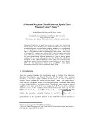
<strong>Heuristic</strong> <strong>Methods</strong> <strong>for</strong> <strong>Graph</strong> <strong>Coloring</strong> <strong>Problems</strong><br />
A. Lim, Y. Zhu<br />
Department of IEEM<br />
Hong Kong Univ of Sci & Tech<br />
Clear Water Bay<br />
Kowloon, Hong Kong<br />
{iealim,zhuyi}@ust.hk<br />
Q. Lou<br />
Department of CS<br />
National Univ of Singapore<br />
3 Science Drive 2<br />
Singapore<br />
louqin@comp.nus.edu.sg<br />
B. Rodrigues<br />
School of Business<br />
Singapore Management Univ<br />
469 Bukit Timah Road<br />
Singapore<br />
br@smu.edu.sg<br />
ABSTRACT<br />
In this work, the <strong>Graph</strong> <strong>Coloring</strong> Problem and its generalizations<br />
- the Bandwidth <strong>Coloring</strong> Problem, the Multicoloring<br />
Problem and the Bandwidth Multicoloring Problem<br />
- are studied. A Squeaky Wheel Optimization with Tabu<br />
Search heuristic is developed and experiments using benchmark<br />
geometric test cases show that the algorithm per<strong>for</strong>ms<br />
well <strong>for</strong> these problems and achieves results <strong>for</strong> the Bandwidth<br />
Multicoloring Problem which improve on results obtained<br />
by other researchers.<br />
Categories and Subject Descriptors<br />
F.2.2 [Nonnumerical Algorithms and <strong>Problems</strong>]: [Sequencing<br />
and scheduling]<br />
Keywords<br />
<strong>Heuristic</strong>s, Optimization, Tabu Search, <strong>Graph</strong> <strong>Coloring</strong><br />
1. INTRODUCTION<br />
The <strong>Graph</strong> <strong>Coloring</strong> Problem (GCP) is a well-known NPcomplete<br />
problem that has been studied extensively. <strong>Heuristic</strong>s<br />
have been widely used <strong>for</strong> the GCP (see, <strong>for</strong> example,<br />
[1]); these include: iterative Greedy by Culberson and Luo<br />
[3], Tabu Search by Hertz and de Werra [6] and Glover et<br />
al. [5], DSATUR by Brelaz [1], XRLF by Johnson et al<br />
[7]. Other techniques, such as combining of the S-IMPASSE<br />
algorithm with exhaustive search [10] and a distributed coloration<br />
neighborhood search [13] have also been introduced.<br />
Among these, the well-known Greedy method is the simplest<br />
which takes an ordering of nodes of a graph and colors<br />
these with the smallest color satisfying the constraints that<br />
no adjacent nodes are assigned same colors. However, the<br />
Greedy method per<strong>for</strong>ms poorly in practice. DSATUR uses<br />
a heuristic which changes the ordering of nodes and then<br />
uses the Greedy method to color these nodes. Further to<br />
this, exact algorithms, such as branch and bound, have been<br />
used to solve instances with a small number of colors [16].<br />
Permission to make digital or hard copies of all or part of this work <strong>for</strong><br />
personal or classroom use is granted without fee provided that copies are<br />
not made or distributed <strong>for</strong> profit or commercial advantage and that copies<br />
bear this notice and the full citation on the first page. To copy otherwise, to<br />
republish, to post on servers or to redistribute to lists, requires prior specific<br />
permission and/or a fee.<br />
SAC’05, March 13-17, 2005, Santa Fe, New Mexico, USA.<br />
Copyright 2005 ACM 1-58113-964-0/05/0003...$5.00.<br />
Most of the early work done on this problem can be found<br />
in: “Cliques, <strong>Coloring</strong> and Satisfiability, Second DIMACS<br />
Implementation Challenge” [8].<br />
The Multi-<strong>Coloring</strong> Problem (with weighted nodes), the<br />
Bandwidth <strong>Coloring</strong> Problem (with weighted edges) and the<br />
Bandwidth Multi-<strong>Coloring</strong> Problem (with weighted edges<br />
and nodes) are generalizations of the GCP and have a range<br />
of applications. The Multi-<strong>Coloring</strong> Problem can be used,<br />
<strong>for</strong> example, to schedule jobs with different time requirements<br />
where the set of colors assigned to a node corresponds<br />
to resources (e.g. men) assigned to a job. Here, each node<br />
has a demand of a set of colors which we have to assign to it<br />
ensuring that its neighbors receive disjoint sets (e.g. sets of<br />
men). A related application is in scheduling processor tasks<br />
where certain resources cannot be shared concurrently by<br />
certain sets of jobs. The problem of channel frequency assignment<br />
arises with different transmitters operating in the<br />
same region which can interfere with each other. This is<br />
common to mobile or general radio networks. The problem<br />
can be viewed as a multicoloring problem where each node<br />
of an interference graph has an associated integer weight<br />
representing the number of calls that must be served by<br />
the corresponding base station. We then seek to assign the<br />
weighted number of colors to each node such that adjacent<br />
nodes are assigned disjoint sets of colors. The objective is<br />
then to minimize the number of colors used <strong>for</strong> such an assignment.<br />
Because of signal interference in networks, adjacent<br />
transmitters need to operate at different and separated<br />
frequencies. This separation requirement is addressed by<br />
constraining frequencies to be separated by stipulated ”distances”,<br />
usually some positive integer. In such problems,<br />
a ”bandwidth” is associated with each frequency.The Bandwidth<br />
<strong>Coloring</strong> and Multi-<strong>Coloring</strong> <strong>Problems</strong> have been used<br />
<strong>for</strong> channel frequency assignment with interference problems.<br />
In the Fixed Channel Assignment Problem [14], <strong>for</strong><br />
example, frequency demand is <strong>for</strong>ecasted and used to determine<br />
network requirements and frequencies are assigned<br />
in advance. In this problem, each cell requires a single assigned<br />
frequency and the Bandwidth <strong>Coloring</strong> Problem can<br />
be used. In general, when cells require a number of separated<br />
frequencies, the Bandwidth Multi-<strong>Coloring</strong> Problem is<br />
used. For example, this problem can be applied to the Fixed<br />
Channel Assignment Problem when co-channel constraints,<br />
adjacent channel constraints and the co-site constraints are<br />
included [14].<br />
Recently, Prestwich proposed a combination of local search<br />
and constraint propagation in a method called FCNS to<br />
solve generalized graph coloring problems [15]. This ap-<br />
933
proach is a hybrid of the DSATUR backtracker and the<br />
S-IMPASSE local search algorithm and was applied in experiments<br />
to geometric graphs. More recently, Lim et al.<br />
proposed a hybrid method which combines Squeaky Wheel<br />
Optimization (SWO) and hill-climbing techniques which was<br />
also tested on geometric graphs [12]. Squeaky Wheel Optimization<br />
(SWO) is a meta-heuristic in which the core is a<br />
Construct-Analyze-Prioritize cycle [2, 9], which we will introduce<br />
in details in Section 3.3. In this work, we propose<br />
new algorithms which use Tabu Search and SWO. In particular,<br />
the SWO with Tabu Search hybrid allows SWO diversification<br />
to be complemented by Tabu Search intensification<br />
in search. We found that this approach gives superior results<br />
when compared with those obtained by Prestwich and Lim<br />
et al. [15, 12] in the Bandwidth Multi-<strong>Coloring</strong> Problem<br />
which is the most difficult of those compared.<br />
This paper is organized as follows. In Section 2, we will<br />
give definitions of the GCP and its generalizations - the<br />
Bandwidth <strong>Coloring</strong> Problem, the Multi-<strong>Coloring</strong> Problem<br />
(MCP) and the Bandwidth MCP. In Section 3, we will describe<br />
the algorithm, its framework and each of its components<br />
- a Greedy Algorithm, SWO and Tabu Search. In<br />
Section 4, we will present experimental results with comparisons<br />
and analysis. In the last section, we will provide a<br />
conclusion.<br />
2. PROBLEM DESCRIPTIONS<br />
We give brief descriptions of the problems we study here.<br />
2.1 The <strong>Graph</strong> <strong>Coloring</strong> Problem<br />
Problem: Given a graph G(V,E), find a minimum k,<br />
and a mapping r : V →{1, ..., k} such that r(i) ≠ r(j) <strong>for</strong><br />
each edge (i, j) ∈ E.<br />
This is the classical problem when each node in the graph<br />
is assigned one color and colors <strong>for</strong> adjacent nodes must be<br />
different. Many practical applications can be modelled as<br />
GCPs, as we mentioned above. This problem has been wellstudied.<br />
In this problem, each node can only be assigned one<br />
color and there are no “distance” restrictions <strong>for</strong> adjacent<br />
nodes. The GCP can be extended as in the following.<br />
2.2 The Bandwidth <strong>Coloring</strong> Problem<br />
Problem: Given a graph G(V,E) with edge weights d(i, j),<br />
find a minimum k and a mapping r from V → {1, ..., k}<br />
such that r(i) ≠ r(j) and |r(i) − r(j)| ≥d(i, j) <strong>for</strong> each edge<br />
(i, j) ∈ E.<br />
In this model, the additional constraint that the distance<br />
between r(i) and r(j) is at least d(i, j) <strong>for</strong> each edge can<br />
be used to model certain applications, such as channel assignment<br />
problem, where edge weights are interpreted as<br />
the minimum required “separation distance” between two<br />
adjacent stations, cells, etc.<br />
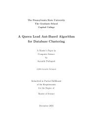
2.3 The Multi-<strong>Coloring</strong> Problem<br />
Problem: Given a graph G(V,E) with node weights<br />
k(i) <strong>for</strong> each i ∈ V , find a minimum k and subsets S(i)<br />
⊂ {1, ..., k} such that |S(i)| = k(i) <strong>for</strong> each i ∈ V and<br />
S(i) ∩ S(j) =∅ <strong>for</strong> each (i, j) ∈ E (where |A| denotes the<br />
cardinality of set A)<br />
In this model, each node can be assigned multiple colors.<br />
Figure 1 is an example of a valid Multi-<strong>Coloring</strong> instance<br />
with k =8.<br />
5 6<br />
K = 2<br />
1 2 3 4<br />
K = 4<br />
K = 4<br />
5 6 7 8<br />
K = 3<br />
1 2 3<br />
Figure 1: An instance of the Multi-coloring Problem<br />
6 9<br />
d = 3<br />
K = 2<br />
d = 1<br />
d = 2<br />
d = 3<br />
1 2 3 4<br />
d = 2<br />
K = 4<br />
d = 1<br />
d = 2<br />
K = 4<br />
5 7 9 11<br />
K = 3<br />
1 3 13<br />
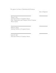
Figure 2: An instance of the Bandwidth Multicoloring<br />
Problem<br />
2.4 The Bandwidth Multi-<strong>Coloring</strong> Problem<br />
Problem: Given a graph G(V,E) with node weights k(i)<br />
<strong>for</strong> i ∈ V , and edge weights d(i, j) <strong>for</strong> (i, j) ∈ E, find a<br />
minimum k and subsets S(i) ⊂{1, ..., k} <strong>for</strong> each i ∈ V , such<br />
that |S(i)| = k(i) <strong>for</strong> each i ∈ V and such that S(i)∩S(j) =<br />
∅ and where, <strong>for</strong> each p ∈ S(i) and q ∈ S(j), |p − q| ≥d(i, j)<br />
<strong>for</strong> each (i, j) ∈ E.<br />
This model combines the above two models, and is more<br />
complex. Note that the graph can contain self-loops. For<br />
example, d(1, 1) = 2,k(1) = 3 means the 3 colors assigned<br />
to node 1 must have a difference of value 2 at least between<br />
any two of them. The example given in Figure 1 is not a<br />
valid bandwidth Multi-<strong>Coloring</strong> instance since it violates the<br />
bandwidth constraint. The example given in Figure 2 is an<br />
example of a valid instance of the problem.<br />
3. A HEURISTIC APPROACH<br />
In this section, we discuss a heuristic approach to tackle<br />
generalized graph coloring problems. Since the Bandwidth<br />
MCP is a generalization of the other three problems, we<br />
apply the algorithm only to it.<br />
We will first present the framework of the approach, then<br />
discuss its components — Greedy Algorithm, SWO and<br />
Tabu Search (TS) respectively.<br />
3.1 Algorithm Framework<br />
In the algorithm, we modeled solutions as sequences of<br />
nodes. Given a sequence of “problem elements”, in the context<br />
of the SWO approach, we used a greedy algorithm to assign<br />
colors to it <strong>for</strong> a solution and then apply meta-heuristics<br />
to adjust these sequences to achieve good or better solutions.<br />
Here, the nodes in the graph are the natural candidates to<br />
d = 2<br />
934
3<br />
k = 2<br />
2<br />
k = 1<br />
2<br />
3<br />
2<br />
k = 3<br />
2<br />
Split<br />
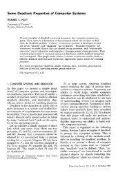
Figure 3: A Instance <strong>for</strong> Splitting the Nodes in the<br />
<strong>Graph</strong><br />
Initial Sequence<br />
SWO<br />
Sequence<br />
Greedy Algorithm<br />
Solution<br />
Best Sequence<br />
Solution<br />
3<br />
Sequence<br />
2<br />
2<br />
TS / SA<br />
3<br />
2<br />
2<br />
2<br />
Final Solution<br />
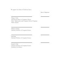
Figure 4: The Framework of the <strong>Heuristic</strong> Approach<br />
be “problem elements” <strong>for</strong> the GCP. However, in the Bandwidth<br />
MCP, this is not easily applied because each node will<br />
be assigned several different colors, between which there are<br />
constraints. To deal with this, we split a node with weight<br />
k into k nodes (except k = 1), and treated each new node as<br />
the “problem element” in the context of SWO. Hence, node i<br />
with weight k becomes a k−clique (a complete subgraph) in<br />
the new graph, with each edge having weight d(i, i) which<br />
was originally the loop edge weight. This process is illustrated<br />
in Figure 3. If the original graph had n nodes and<br />
node i had weight k(i), 1 ≤ i ≤ n, then the new graph will<br />
have P n<br />
i=1<br />
k(i) nodes.<br />
When a sequence is given, it will be passed to the greedy<br />
algorithm to generate a solution. The greedy algorithm<br />
is “deterministic” or one-one correspondence, i.e., <strong>for</strong> two<br />
identical sequences, resulting solutions are the same. This<br />
allowed us to exploit meta-heuristic to adjust sequences to<br />
find good or better solutions.<br />
The algorithm can be divided into two parts. In the first<br />
part, the SWO technique is applied to adjust sequences globally,<br />
in particular, through diversification. From this, the<br />
best solution that SWO finds is passed to a TS heuristic <strong>for</strong><br />
refinement and better solutions. We adopted TS as the second<br />
meta-heuristics here because of its strength in searching<br />
<strong>for</strong> good solutions in a local search space while avoiding local<br />
optima.<br />
The greedy algorithm will then be invoked to evaluate the<br />
sequence so as to determine the number of colors it requires.<br />
The entire framework is summarized in Figure 4.<br />
3.2 The Greedy Algorithm<br />
The greedy algorithm takes a sequence of “split nodes”<br />
and assign colors to them greedily. The idea is straight<strong>for</strong>ward.<br />
Following the node sequence, we assign colors one by<br />
one where, <strong>for</strong> each node, we assign the smallest possible<br />
color not used by adjacent earlier nodes. The details of this<br />
algorithm is shown as Algorithm 1. Here,<br />
n is the number of nodes in the original graph;<br />
d(i, j) is the weight of edge (i, j);<br />
m is the number of nodes after splitting;<br />
p[1..m] is the priority sequence <strong>for</strong> the m nodes (p[1] = u<br />
935<br />
implies node u has the highest priority);<br />
c[1..m] records the assigned colors.<br />
and the function get original node(u) returns the node v<br />
in the original graph such that u is split from v.<br />
Algorithm 1 The Greedy Algorithm which Assigns Colors<br />
<strong>for</strong> i =1tom do<br />
c[i] ←−1<br />
end <strong>for</strong><br />
<strong>for</strong> i =1tom do<br />
<strong>for</strong>bidden set ←∅<br />
u ← p[i]<br />
v ← get original node(u)<br />
<strong>for</strong> each node s that adjacent to u do<br />
if c[s]! = −1 then<br />
t ← get original node(s)<br />
a ← Max{0,c[s] − d(v, t)+1}<br />
b ← c[s]+d(v, t) − 1<br />
<strong>for</strong>bidden set ← <strong>for</strong>bidden set ∪ [a..b]<br />
end if<br />
end <strong>for</strong><br />
c[u] ← Min{r, r ∈ N,r /∈ <strong>for</strong>bidden set}<br />
end <strong>for</strong><br />
3.3 Squeaky Wheel Optimization<br />
“Squeaky Wheel” Optimization (SWO) is a meta-heuristic<br />
in which the core is a Construct-Analyze-Prioritize cycle [2,<br />
9]. A solution is constructed by a constructor using a<br />
greedy algorithm where decisions are determined by the priorities<br />
assigned to the elements of the problem. The analyzer<br />
then takes over and is the component that looks <strong>for</strong><br />
those elements that are ”trouble makers” and assigns numerical<br />
“blame” values to these problem elements i.e. those<br />
elements that contribute to weaknesses in the current solution.<br />
In [9], blames are assigned to the nodes that use new<br />
colors, <strong>for</strong> example. A prioritizer will then modify the sequence<br />
of problem elements and increase the priorities of the<br />
trouble makers which then causes the constructor to process<br />
them earlier in the next iteration. The cycle repeats until<br />
a specified termination condition (number of iterations) is<br />
satisfied.<br />
The SWO technique has been successful in applications<br />
to Machine Scheduling and <strong>Graph</strong> <strong>Coloring</strong> <strong>Problems</strong> [2, 9].<br />
Here we used SWO to generate an initial solution. One reason<br />
<strong>for</strong> this choice is that SWO is fast when compared with<br />
other meta-heuristics such as TS, Simulated Annealing and<br />
Genetic Algorithms. The other reason is that SWO is able<br />
explore the search space more widely and can provide <strong>for</strong><br />
good diversification in search. It considers both the solution<br />
space and the priority space where small changes in the<br />
priority space can cause a large change in solution space.<br />
This property causes SWO to view the solution space more<br />
globally. The components of SWO, the constructor, the<br />
analyzer and the prioritizer, are described as follows:<br />
• The Constructor: A greedy algorithm is invoked.<br />
The priority sequence of the “problem elements” - the<br />
split nodes - is passed to the algorithm and a corresponding<br />
greedy solution constructed.<br />
• The Analyzer: The analyzer will identify the socalled<br />
“trouble makers” and assign blame values to<br />
them.
• The Prioritizer: Once blame has been assigned, the<br />
prioritizer modifies the previous sequence of problem<br />
elements. The nodes with higher blame values will be<br />
moved <strong>for</strong>ward in the priority sequence while the ones<br />
with small blame values will remain in the back of<br />
the sequence. This causes the “trouble makers” to be<br />
handled first by the constructor in the next iteration.<br />
Here, we used a new scheme to calculate the blame values<br />
<strong>for</strong> the implementation of SWO. Assume that, in the current<br />
solution, the maximum color is K. We define “trouble<br />
makers” as those elements that use colors which are “large<br />
enough”. If the node is assigned color c, then c is “large<br />
enough” if c > α.K, where α is a real number (called a<br />
blame rate) in (0, 1) and close to 1. Problem elements will<br />
be assigned a constant blame value b.<br />
The SWO algorithm is described in Algorithm 2.<br />
Algorithm 2 The SWO procedure<br />
Initialize a random priority sequence pri<br />
max value ←∞<br />
<strong>for</strong> i = 1 to maximum SWO iterations do<br />
invoke the greedy algorithm with the sequence pri<br />
cur value ← the maximum color in the current solution<br />
if cur value < max value then<br />
max value ← cur value<br />
update best solution<br />
end if<br />
<strong>for</strong> j=1 to m do<br />
blame[j] ← j<br />
if c[j] >α∗ cur value then<br />
blame[j] ← blame[j]+b<br />
end if<br />
end <strong>for</strong><br />
sort the sequence pri in ascending order of blame values<br />
end <strong>for</strong><br />
We first ran the SWO <strong>for</strong> a number of iterations and<br />
picked up the best solution to be the initial solution of TS,<br />
which we discuss in the next section.<br />
3.4 Tabu Search<br />
TS is iterative method designed to help standard local<br />
search methods escape local optima operating through neighborhood<br />
moves that proceed from one solution to another<br />
at each iteration. In basic TS, some moves are tabu and<br />
<strong>for</strong>bidden unless they lead to desirable outcomes [4].<br />
As mentioned earlier, we only considered sequences of<br />
problem elements (split nodes). The neighborhood move<br />
is an exchange of two nodes in the solution sequence. The<br />
move can be denoted a ↔ b <strong>for</strong> 1 ≤ a, b ≤ m, where m is<br />
the number of nodes in the graph after splitting. A tabu<br />
memory is used to <strong>for</strong>bid a reverse move, within a certain<br />
number of iterations, to avoid traps at local optima and the<br />
number of iterations <strong>for</strong> which a particular restriction remains<br />
is given by a tabu tenure. Taking iter to denote the<br />
current iteration, after we select the move a ↔ b as the best<br />
one from a number of neighborhood moves (specified as No.<br />
TS moves in the next section), tabu memory is updated as<br />
tabu (a, b) =iter + tabu tenure. The reverse move b ↔ a is<br />
then prevented in the next tabu tenure number of iterations.<br />
The TS procedure is detailed in Algorithm 3.<br />
Algorithm 3 The Tabu Search Procedure<br />
get initial solution x now from SWO method<br />
x best ← x now<br />
iter ← 0<br />
while iter ≤ max iter do<br />
generate the neighborhood set N(x now) by the exchange<br />
move<br />
evaluate each candidate solution x trial as f(x trial ), by<br />
the greedy algorithm<br />
x next ←∅<br />
<strong>for</strong> all x trial exchanging elements a and b do<br />
if iter > tabu(a ↔ b) and f(x next) >f(x trial ) then<br />
x next ← x trial<br />
p ← a, q ← b<br />
end if<br />
end <strong>for</strong><br />
tabu(p ↔ q) ← iter + tabu tenure<br />
x now ← x next<br />
if f(x best ) >f(x now ) then<br />
x best ← x now<br />
end if<br />
iter ← iter +1<br />
end while<br />
4. EXPERIMENTAL RESULTS<br />
To test the algorithms, we used the 33 benchmark geometric<br />
instances given by Trick which can be found in Computational<br />
Symposium Announcement: <strong>Graph</strong> <strong>Coloring</strong> and its<br />
Generalizations at http://mat.gsia.cmu.edu/COLORING02/.<br />
Points are generated in a 10,000 by 10,000 grid and are connected<br />
by an edge if they are close enough together. Edge<br />
weights are inversely proportional to the distance between<br />
nodes and node weights are uni<strong>for</strong>mly generated. GEOMn<br />
instances are sparse; GEOMa and GEOMb instances are<br />
denser and require fewer colors per node.<br />
We implemented the SWO+TS algorithm using Java and<br />
with the results, we list those from [15] and [11], <strong>for</strong> experiments<br />
on the same set of instances.<br />
Table 1 gives the parameter settings <strong>for</strong> the four problems.<br />
We experimented with different number of restarts<br />
and found that after 10 restarts the marginal improvement<br />
was small (with a maximum of 2 colors in only two cases out<br />
of 33), and beyond 15 restarts, the improvement was negligible.<br />
With more restarts, however, running times increased.<br />
We there<strong>for</strong>e chose to restart the algorithm 10 times with<br />
different (randomized) initial solutions. The comparisons<br />
between the method and the previous two methods is shown<br />
in Table 2 where the following notations are used:<br />
• M1 - Method used by Prestwich [15] 1<br />
• M2 - Method used by Lim et al. [11] 2<br />
• M3 - The SWO+TS method 3<br />
Table 3 and Table 4 give detailed results <strong>for</strong> the MCP and<br />
Bandwidth MCP (The detailed results of GCP and Band-<br />
1 The benchmark program dfmax(r500.5.b) running time:<br />
35.21 seconds (user time).<br />
2 The benchmark program dfmax(r500.5.b) running time:<br />
25.32 seconds (user time).<br />
3 The benchmark program dfmax(r500.5.b) running time:<br />
74.12 seconds (user time).<br />
936
Parameters Pure <strong>Coloring</strong> Bandwidth <strong>Coloring</strong> MCP Bandwidth MCP<br />
Restarts No. 10 10 10 10<br />
SWO Iteration 200 400 400 400<br />
Blame Rate α 0.95 0.95 0.95 0.95<br />
Blame Value b 4 4 4 8<br />
TS Iteration 100 100 200 200<br />
No. of TS Moves 40 40 50 50<br />
TS Tenure 5 5 5 5<br />
1 Not presented in [15]<br />
Table 1: Parameter Settings<br />
Pure <strong>Coloring</strong> Bandwidth <strong>Coloring</strong> MCP Bandwidth MCP<br />
M1 M2 M1 M2 M1 1 M2 M1 2 M2<br />
Wins 0 0 0 17 - 0 16 22<br />
Ties 30 31 15 14 - 33 1 11<br />
Loses 3 2 18 2 - 0 0 0<br />
Max Wins 0 0 0 5 - 0 77 11<br />
Avg. Wins 0 0 0 1.53 - 0 20.75 5.23<br />
Max Loses 1 1 11 2 - 0 0 0<br />
Avg. Loses 1.00 1.00 4.61 1.50 - 0 0 0<br />
2 Only 17 instances presented in [15]<br />
Table 2: Comparison of M3 with M1 and M2<br />
width <strong>Coloring</strong> are not presented here due to the space limitation),<br />
where k denotes the number of colors and t denotes<br />
the running time in seconds. In [15], when there are no<br />
results <strong>for</strong> the MCP, and only partial results <strong>for</strong> the Bandwidth<br />
MCP, we write “-” in the tables to denote this.<br />
The per<strong>for</strong>mance of the algorithms is good in all four problems<br />
and especially so <strong>for</strong> the Bandwidth MCP. We conducted<br />
the experiments using Bandwidth MCP instances<br />
which are not covered in [15]. Results tied or surpassed all<br />
of the results in [15] and [11]. Although the methods that<br />
are applied in [15] are good <strong>for</strong> GCP and per<strong>for</strong>m well on<br />
the DIMACS geometric graph instances, the new algorithm<br />
is only weaker in 3 out of 33 cases and <strong>for</strong> only 1 color each.<br />
In the Bandwidth <strong>Coloring</strong> Problem, results are not as good<br />
as [15] although comparable with [11].<br />
We believe that the method in [15] does not work well <strong>for</strong><br />
the Bandwidth MCP because there are too many variables<br />
and constraints to check simultaneously. The backtracker<br />
used there would take a long time to deal with the many<br />
constraints. However, the approach given in [11] and here<br />
always generates a solution quickly and then improves on it<br />
incrementally. One of the reasons why the method outper<strong>for</strong>ms<br />
[11] is that TS works well with SWO and is able to<br />
avoid local optima. Furthermore, we used TS after SWO,<br />
whereas hill-climbing was implemented in each iteration of<br />
the SWO in [11] which results in longer times. In the same<br />
amount of time, we were able to run more iterations of SWO<br />
to refine the solutions.<br />
It is interesting that in the MCP, we obtained the same<br />
results as [11] on all the 33 instances. No results are provided<br />
in [15] <strong>for</strong> this problem.<br />
In terms of running time, the method takes relatively<br />
longer times <strong>for</strong> small instances, especially <strong>for</strong> the <strong>Coloring</strong><br />
and Bandwidth <strong>Coloring</strong>. However, the running times<br />
did not increase sharply when instances became larger, and<br />
are comparable with the other two methods. We believe<br />
this is due to the different heuristics setup. Since we used<br />
constant parameters, running times will not change much<br />
as the sizes vary; however, the running times of the other<br />
heuristics were dependant on the instance sizes.<br />
5. CONCLUSION<br />
In this work, we discussed several variations of generalized<br />
graph coloring problems and proposed a new hybrid<br />
SWO with TS technique to solve these. Experiments are<br />
conducted using benchmark problems and results compared<br />
with those obtained by existing methods. These results show<br />
that this approach is effective <strong>for</strong> the problems studied and<br />
provides superior results than the current methods <strong>for</strong> the<br />
Bandwidth MCP.<br />
6. REFERENCES<br />
[1] D. Brelaz. New methods to color the vertices of a<br />
graph. Communications of ACM, 22(4):251–256, 1979.<br />
[2] David P. Clements, James M. Craw<strong>for</strong>d, David E.<br />
Joslin, Geoge L. Nemhauser, Markus E. Puttlitz, and<br />
Martin W.P. Savelsbergh. Heurstic optimization: A<br />
hybrid ai/or approach. In Proceedings of the Workshop<br />
on Industrial Constraint-Directed Scheduling, 1997.<br />
[3] Joseph C. Culberson and Feng Luo. Exploring the<br />
k-colorable landscape with iterative greedy. Cliques,<br />
<strong>Coloring</strong> and Satisfiability, Second DIMACS<br />
Implementation Challenge, 1993.<br />
[4] Fred Glover and Manuel Laguna. Tabu Search. Kluwer<br />
Acadamic Publishers, 1997.<br />
[5] Fred Glover, Mark Parker, and Jennifer Ryan.<br />
<strong>Coloring</strong> by tabu branch and bound. Cliques, <strong>Coloring</strong><br />
937
and Satisfiability, Second DIMACS Implementation<br />
Challenge, 1993.<br />
[6] A. Hertz and D. de Werra. Using tabu search<br />
techniques <strong>for</strong> graph coloring. Computing, 39:345–351,<br />
1987.<br />
[7] D. S. Johnson, C. A. Aragon, L. A. Mcgeoch, and<br />
C. Schevon. Optimization by simulated annealing: An<br />
experimental evaluation c part ii (graph coloring and<br />
number partitioning). Operations Research,<br />
31:378–406, 1991.<br />
[8] David S. Johnson and Michael A. Trick (Editors).<br />
Cliques, <strong>Coloring</strong> and Satisfiability, Second DIMACS<br />
Implementation Challenge. American Mathematical<br />
Society, 1993.<br />
[9] David E. Joslin and David P. Clements. “squeaky<br />
wheel” optimization. In Proceedings of American<br />
Association of Artificial Intelligence National<br />
Conference 1998, pages 340–346, 1998.<br />
[10] Gray Lewandowski and Anne Condon. Expreiments<br />
with parallel graph coloring heuristics and applications<br />
of graph coloring. Cliques, <strong>Coloring</strong> and Satisfiability,<br />
Second DIMACS Implementation Challenge, 1993.<br />
[11] Andrew Lim, Brian Rodrigues, and Yi Zhu. Crane<br />
scheduling using swo with local search. In Proceedings<br />
of 4th Asia-Pacific Conference on Simulated Evolution<br />
and Learning, 2002.<br />
[12] Andrew Lim, Xingwen Zhang, and Yi Zhu. A hybrid<br />
method <strong>for</strong> the graph coloring problem and its<br />
generalizations. In 5th Metaheuristics International<br />
Conference (MIC 2003), 2002.<br />
[13] Craig Morgenstern. Distributed coloration<br />
neighborhood search. Cliques, <strong>Coloring</strong> and<br />
Satisfiability, Second DIMACS Implementation<br />
Challenge, 1993.<br />
[14] Eun-Jon Park, Yong-Hyuk Kim, and Byung-Ro Moon.<br />
Genetic search <strong>for</strong> fixed channel assignment problem<br />
with limited bandwidth. In Proceedings of Genetic and<br />
Evolutionary Computation Conference, pages<br />
1772–1779, 2002.<br />
[15] Steven Prestwich. Constrained bandwidth<br />
multicoloration neighborhoods. In Proceedings of<br />
Computational Symposium on <strong>Graph</strong> <strong>Coloring</strong> and its<br />
Generalizations, 2002.<br />
[16] E. C. Sewell. An improved algorithm <strong>for</strong> exact graph<br />
coloring. Cliques, <strong>Coloring</strong> and Satisfiability, Second<br />
DIMACS Implementation Challenge, 1993.<br />
938
<strong>Graph</strong> M1 M2 M3 <strong>Graph</strong> M1 M2 M3<br />
k t k t k t k t k t k t<br />
GEOM20 - - 28 0 28 4 GEOM80 - - 63 0 63 551<br />
GEOM20a - - 30 0 30 3 GEOM80a - - 68 0 68 476<br />
GEOM20b - - 8 0 8 7 GEOM80b - - 25 0 25 111<br />
GEOM30 - - 26 0 26 61 GEOM90 - - 51 0 51 697<br />
GEOM30a - - 40 0 40 99 GEOM90a - - 65 0 65 625<br />
GEOM30b - - 11 0 11 20 GEOM90b - - 28 0 28 135<br />
GEOM40 - - 31 0 31 131 GEOM100 - - 60 0 60 845<br />
GEOM40a - - 46 0 46 138 GEOM100a - - 81 0 81 854<br />
GEOM40b - - 14 0 14 29 GEOM100b - - 30 0 30 156<br />
GEOM50 - - 35 0 35 227 GEOM110 - - 62 0 62 1022<br />
GEOM50a - - 61 0 61 312 GEOM110a - - 91 0 91 1172<br />
GEOM50b - - 17 0 17 46 GEOM110b - - 37 0 37 211<br />
GEOM60 - - 36 0 36 275 GEOM120 - - 64 0 64 1268<br />
GEOM60a - - 65 0 65 391 GEOM120a - - 93 0 93 2349<br />
GEOM60b - - 22 0 22 64 GEOM120b - - 34 0 34 489<br />
GEOM70 - - 44 0 44 374<br />
GEOM70a - - 71 0 71 439<br />
GEOM70b - - 22 0 22 84<br />
Table 3: Experimental Results <strong>for</strong> MCP<br />
<strong>Graph</strong> M1 M2 M3 <strong>Graph</strong> M1 M2 M3<br />
k t k t k t k t k t k t<br />
GEOM20 159 56 149 0 149 176 GEOM80 - - 394 4041 383 2159<br />
GEOM20a 175 145 169 16 169 169 GEOM80a - - 379 677 379 2006<br />
GEOM20b 44 25 44 0 44 25 GEOM80b 152 1380 145 3230 141 417<br />
GEOM30 168 178 160 0 160 241 GEOM90 - - 335 4095 332 2623<br />
GEOM30a 235 64 211 10 209 425 GEOM90a - - 382 10404 377 2587<br />
GEOM30b 79 14 77 0 77 69 GEOM90b - - 157 648 157 489<br />
GEOM40 189 135 167 3 167 496 GEOM100 - - 413 631 404 3283<br />
GEOM40a 260 24 214 358 213 573 GEOM100a - - 462 172 459 3529<br />
GEOM40b 80 94 76 8 74 108 GEOM100b - - 172 4893 170 584<br />
GEOM50 257 96 224 41 224 819 GEOM110 - - 389 577 383 3893<br />
GEOM50a 395 299 326 96 318 125 GEOM110a - - 501 4671 494 4661<br />
GEOM50b 89 94 87 53 87 162 GEOM110b - - 210 12 206 716<br />
GEOM60 279 514 258 46 258 1016 GEOM120 - - 409 1825 402 4317<br />
GEOM60a - - 368 3748 358 1717 GEOM120a - - 564 5335 556 6688<br />
GEOM60b 128 1012 119 300 116 246 GEOM120b - - 201 869 199 1028<br />
GEOM70 310 1019 279 25 273 1458<br />
GEOM70a - - 478 417 469 1987<br />
GEOM70b 133 766 124 136 121 312<br />
Table 4: Experimental Results <strong>for</strong> Bandwidth MCP<br />
939