enumeration of self-complementary plane partitions

(−1)–ENUMERATION OF SELF–COMPLEMENTARY PLANE
PARTITIONS
THERESIA EISENKÖLBL
Fakultät für Mathematik, Universität Wien,
Nordbergstraße 15, A-1090 Wien, Austria.
E-mail: Theresia.Eisenkoelbl@univie.ac.at
Abstract. We prove a product formula for the remaining cases of the weighted
enumeration of self–complementary plane partitions contained in a given box where
adding one half of an orbit of cubes and removing the other half of the orbit changes the
weight by −1. We use nonintersecting lattice path families to express this enumeration
as a Pfaffian which can be expressed in terms of the known ordinary enumeration of
self–complementary plane partitions.
1. Introduction
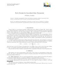
A plane partition P can be defined as a finite set of integer points (i, j, k) with
i, j, k > 0 and if (i, j, k) ∈ P and 1 ≤ i ′ ≤ i, 1 ≤ j ′ ≤ j, 1 ≤ k ′ ≤ k then (i ′ , j ′ , k ′ ) ∈ P .
We interpret these points as midpoints of cubes and represent a plane partition by
stacks of cubes (see Figure 1). If we have i ≤ a, j ≤ b and k ≤ c for all cubes of the
plane partition, we say that the plane partition is contained in a box with sidelengths
a, b, c.
Plane partitions were first introduced by MacMahon. One of his main results is the
following [10, Art. 429, x → 1, proof in Art. 494]:
The number of all plane partitions contained in a box with sidelengths a, b, c equals
B(a, b, c) =
a∏
b∏
c∏
i=1 j=1 k=1
i + j + k − 1
a∏
i + j + k − 2 =
i=1
(c + i) b
(i) b
, (1)
where (a) n := a(a + 1)(a + 2) . . . (a + n − 1) is the rising factorial.
MacMahon also started the investigation of the number of plane partitions with
certain symmetries in a given box. These numbers can also be expressed as product
formulas similar to the one given above. In [14], Stanley introduced additional complementation
symmetries giving six new combinations of symmetries which led to more
conjectures all of which were settled in the 1980’s and 90’s (see [14, 8, 3, 17]).
Many of these theorems come with q–analogs, that is, weighted versions that record
the number of cubes or orbits of cubes by a power of q and give expressions containing
q–rising factorials instead of rising factorials (see [1, 2, 11]). For plane partitions with
complementation symmetry, it seems to be difficult to find natural q–analogs. However,
2000 Mathematics Subject Classification. Primary 05A15; Secondary 05B45 52C20.
Key words and phrases. lozenge tilings, rhombus tilings, plane partitions, determinants, pfaffians,
nonintersecting lattice paths.
111

T. EISENKOEBL
2 THERESIA EISENKÖLBL
Figure 1. A self–complementary plane partition
in Stanley’s paper a q–analog for self–complementary plane partitions is given (the
weight is not symmetric in the three sidelengths, but the result is). Interestingly, upon
setting q = −1 in the various q–analogs, one consistently obtains enumerations of other
objects, usually with additional symmetry restraints. This observation, dubbed the
“’(−1)–phenomenon” has been explained for many but not all cases by Stembridge (see
[15] and [16]).
In [7], Kuperberg defines a (−1)–enumeration for all plane partitions with complementation
symmetry which admits a nice closed product formula in almost all cases.
These conjectures were solved in Kuperberg’s own paper and in the paper [4] except
for one case without a nice product formula and the case of self-complementary plane
partitions in a box with some odd sidelengths which will be the main theorem of this
paper. We start with the precise definitions.
A plane partition P contained in the box a × b × c is called self–complementary if
(i, j, k) ∈ P ⇔ (a + 1 − i, b + 1 − j, c + 1 − k) /∈ P for 1 ≤ i ≤ a, 1 ≤ j ≤ b, 1 ≤ k ≤ c.
This means that the box consists exactly of the plane partition and the image obtained
from it by symmetry with respect to the central point of the box.
A convenient way to look at a self–complementary plane partition is the projection
to the plane along the (1, 1, 1)–direction (see Figure 1). A plane partition contained in
an a × b × c–box becomes a rhombus tiling of a hexagon with sidelengths a, b, c, a, b, c.
It is easy to see that self-complementary plane partitions correspond exactly to those
rhombus tilings with a 180 ◦ rotational symmetry.
The (−1)–weight is defined as follows: A self–complementary plane partition contains
exactly one half of each orbit under the operation (i, j, k) ↦→ (a+1−i, b+1−j, c+1−k).
Let a move consist of removing one half of an orbit and adding the other half. Two
plane partitions are connected either by an odd or by an even number of moves, so it
is possible to define a relative sign. The sign becomes absolute if we assign weight 1 to
the half-full plane partition (see Figure 2).
112

(-1)-ENUMERATION OF SELF-COMPLEMENTARY PLANE PARTITIONS
(−1)–ENUMERATION OF SELF–COMPLEMENTARY PLANE PARTITIONS 3
Figure 2. A plane partition of weight 1.
Therefore, this weight is (−1) n(P ) where n(P ) is the number of cubes in the “left”
half of the box and we want to evaluate ∑ P (−1)n(P ) . For example, the plane partition
in Figure 1 has weight (−1) 10 = 1.
In order to be able to state the result for the (−1)–enumeration more concisely,
Stanley’s result on the ordinary enumeration of self–complementary plane partitions is
needed. It will also be used as a step in the proof of the (−1)–enumeration.
Theorem 1 (Stanley [14]). The number SC(a, b, c) of self–complementary plane partitions
contained in a box with sidelengths a, b, c can be expressed in terms of B(a, b, c)
in the following way:
B ( a
, b+1,
c−1
2 2 2
B ( a+1
2 , b 2 , c 2
where B(a, b, c) = ∏ a (c+i) b
i=1 (i) b
B ( a
, b , c 2
2 2 2)
for a, b, c even,
) (
B
a , b−1,
)
c+1 for a even and b, c odd,
2 2 2
) (
B
a−1
, b , )
c for a odd and b, c even,
2 2 2
is the number of all plane partitions in an a × b × c–box.
Note that a self-complementary plane partition contains exactly half of all cubes in
the box. Therefore, there are no self-complementary plane partitions in a box with
three odd sidelengths.
Now we can express the (−1)–enumeration of self–complementary plane partitions in
terms of SC(a, b, c), the ordinary enumeration of self–complementary plane partitions.
113

4 THERESIA EISENKÖLBL
Theorem 2. The enumeration of self–complementary plane partitions in a box with
sidelengths a, b, c counted with weight (−1) n(P ) equals
( a
B
2 , b 2 2)
, c )
SC ( a
, b+1,
) ( c−1
2 2 2 SC a , b−1
2
SC ( a+1
2 , b 2 , c 2
, c+1
2 2
)
SC
( a−1
2 , b 2 , c 2
T. EISENKOEBL
)
for a, b, c even,
for a even and b, c odd
for a odd and b, c even
where SC(a, b, c) is given in Theorem 1 in terms of the numbers of plane partitions
contained in a box and n(P ) is the number of cubes in the plane partition P that are
not in the half-full plane partition (see Figure 2).
Remark. Since the sides of the box play symmetric roles this covers all cases. (For
three odd sidelengths there are no self-complementary plane partitions.) The case of
three even sidelengths has already been proved in [4].
Note that Theorem 1 and Theorem 2 are very analogous. In the even case, the (−1)–
enumeration is the square root of the ordinary enumeration. In the other cases, it is
still true that there are half as many linear factors in the (−1)–enumeration (viewed as
a polynomial in c, say).
In Stanley’s paper [14], the theorem actually gives a q–enumeration of plane partitions.
The case q = −1 gives the same expression as Theorem 2 above if at least one
side has odd length, but this does not give a proof of Theorem 2 because the weights of
individual plane partitions are different. In the case of only even sidelengths, Stanley’s
theorem gives SC (a/2, b/2, c/2) 2 (analogously to Theorem 1) which does not equal the
result B (a/2, b/2, c/2) in Theorem 2.
Stanley’s proof uses a special case of the Littlewood-Richardson rule, the expansion
of the product of Schur functions s λ (x 1 , . . . , x n ) · s µ (x 1 , . . . , x n ) where λ and µ are
rectangular partitions whose sidelengths differ by at most one. It is possible to give an
alternative proof of Theorem 2 using a modification of Stanley’s weight leading to the
expansion of s λ (x 1 , . . . , x n+1 ) · s µ (x 1 , . . . , x n ) where λ and µ are rectangular partitions.
(Note the different numbers of variables.) See also the remark at the end of the paper.
2. Outline of the proof
For brevity, we just give the proof in the case a even, b, c odd and (c − b)/2 even.
Step 1: From plane partitions to families of nonintersecting lattice paths.
We use the projection to the plane along the (1, 1, 1)–direction and get immediately
that self–complementary plane partitions contained in an a × b × c–box are equivalent
to rhombus tilings of a hexagon with sides a, b, c, a, b, c invariant under 180 ◦ –rotation.
A tiling of this kind is clearly determined by one half of the hexagon.
Since the sidelengths a, b, c play a completely symmetric role and two of them must
have the same parity we assume without loss of generality that c − b is even and b ≤ c.
The result turns out to be symmetric in b and c, so we can drop the last condition
in the statement of Theorem 2. Write x for the positive integer (c − b)/2 and divide
the hexagon in half with a line parallel to the side of length a (see Figure 3). As
shown in the same figure, we find a bijection between these tiled halves and families of
nonintersecting lattice paths.
114

(-1)-ENUMERATION OF SELF-COMPLEMENTARY PLANE PARTITIONS
(−1)–ENUMERATION OF SELF–COMPLEMENTARY PLANE PARTITIONS 5
⎧
⎪⎨
b
⎪⎩
{
x
⎪⎩
a
⎪⎭
⎪⎨
⎧⎫⎪ ⎬
⎪ ⎭
⎪⎬
a + b
c − x
⎫
• • • ◦• • • •
• • ◦• • • • ◦•
• ◦• • • • ◦• •
◦• • • • • • •
• • • ◦• • • •
• • ◦• • • • •
A 1
A 2
A 3
A 4
E 2
E 3
E 5
E 6
• • • • • • •
Figure 3. The paths for the self–complementary plane partition in Figure
1 and the orthogonal version. (x = c−b
2 )
The starting points of the lattice paths are the midpoints of the edges on the side of
length a. The end points are the midpoints of the edges parallel to a on the opposite
boundary. This is a symmetric subset of the midpoints on the cutting line of length
a + b.
The paths always follow the rhombi of the given tiling by connecting midpoints of
parallel rhombus edges. It is easily seen that the resulting paths have no common points
(i.e. they are nonintersecting) and the tiling can be recovered from a nonintersecting
lattice path family with unit diagonal and down steps and appropriate starting and
end points. Of course, the path families will have to be counted with the appropriate
(−1)–weight.
After changing to an orthogonal coordinate system (see Figure 3), the paths are
composed of unit South and East steps and the coordinates of the starting points are
A i = (i − 1, b + i − 1) for i = 1, . . . , a. (2)
The end points are a points chosen symmetrically among
E j = (x + j − 1, j − 1) for j = 1, . . . , a + b. (3)
Here, symmetrically means that if E j is chosen, then E a+b+1−j must be chosen as well.
Note that the number a + b of potential end points on the cutting line is always odd.
Therefore, there is a middle one which is in no path family for even a (see Figure 3).
Now the (−1)–weight has to be defined for the paths. For a path from A i to E j we
can use the weight (−1) area(P ) where area(P ) is the area between the path and the x–
axis and then multiply the weights of all the paths in the family. We have to check that
the weight changes sign if we replace a half orbit with the complementary half orbit. If
one of the affected cubes is completely inside the half shown in Figure 3, ∑ P area(P )
changes by one. If the two affected cubes are on the border of the figure, two symmetric
endpoints, say E j and E a+b+1−j , are changed to E j+1 and E a+b−j or vice versa. It is
easily checked that in this case ∑ P
area(P ) changes by j + (a + b − j) which is odd.
115

6 THERESIA EISENKÖLBL
It is straightforward to check that the weight for the “half-full” plane partition (see
Figure 2) equals (−1) a(a−2)/8 for a even, b, c odd. Therefore, we have to multiply the
path enumeration by this global sign.
Step 2: From lattice paths to a sum of determinants
This weight can be expressed as a product of weights on individual steps (the exponent
of (−1) is just the height of the step), so the following lemma is applicable. By
the main theorem on nonintersecting lattice paths (see [9, Lemma 1] or [5, Theorem 1])
the weighted count of such families of paths can be expressed as a determinant.
Lemma 3. Let A 1 , A 2 , . . . , A n , E 1 , E 2 , . . . , E n be integer points meeting the following
condition: Any path from A i to E l has a common vertex with any path from A j to E k
for any i, j, k, l with i < j and k < l.
Then we have
P(A → E, nonint.) =
det (P(A i → E j )), (4)
1≤i,j≤n
where P(A i → E j ) denotes the weighted enumeration of all paths running from A i to
E j and P(A → E, nonint.) denotes the weighted enumeration of all families of nonintersecting
lattice paths running from A i to E i for i = 1, . . . , n.
The condition on the starting and end points is fulfilled in our case because the points
lie on diagonals, so we have to find an expression for T ij = P(A i → E j ), the weighted
enumeration of all single paths from A i to E j in our problem.
It is well-known that the enumeration of paths of this kind from (x, y) to (x ′ , y ′ ) is
given by the q–binomial coefficient [ ]
x ′ −x+y−y ′
if the weight of a path is x ′ −x q qe where e is
the area between the path and a horizontal line through its endpoint.
The q–binomial coefficient (see [13, p. 26] for further information) can be defined as
[ ∏ n
n j=n−k+1
=
k]
(1 − qj )
∏ k
j=1 (1 − .
qj )
q
T. EISENKOEBL
Although it is not obvious from this definition, the q–binomial coefficient is a polynomial
in q. So it makes sense to put q = −1.
It is easy to verify that
[ {
n 0 n even, k odd,
= (
k]
⌊n/2⌋
)
(5)
−1
else.
⌊k/2⌋
Taking also into account the area between the horizontal line through the endpoint
and the x–axis, we obtain
[ ] b + x
T ij = P(A i → E j ) = (−1) (x+j−i)(j−1) .
b + i − j
−1
Now we apply Lemma 3 to all possible sets of end points. Thus, the (−1)–enumeration
can be expressed as a sum of determinants which are minors of the a × (a + b)–matrix
T :
Lemma 4. The (−1)–enumeration can be written as
116

(-1)-ENUMERATION OF SELF-COMPLEMENTARY PLANE PARTITIONS
(−1)–ENUMERATION OF SELF–COMPLEMENTARY PLANE PARTITIONS 7
(−1) a(a−2)/8
∑
1≤k 1

8 THERESIA EISENKÖLBL
where T ij = (−1) (x−i)(j−1)[ ]
b+x
b+i−j
−1
(and x = (c − b)/2).
Proof. Apply the lemma with 2m = a, 2n = a + b − 1 and
S = (T 1 , . . . , T a+b−1
2
T. EISENKOEBL
, T a+b+3 , . . . , T a+b )
2
to obtain
⎛
a+b−1
2∑
Pf 1≤i,j≤a
⎝
k=1
⎞
(T ik T j,a+b+1−k − T jk T i,a+b+1−k ) ⎠ .
□
Lemma 7. The Pfaffian for the ordinary enumeration SC(a, b, c) for b ≤ c is
⎛
⌊
⎜
∑
a+b
Pf 1≤i,j≤a ⎝
2 ⌋
k=1
(( b + x
)(
b + x
)
b + i − k j + k − a − 1
−
( )(
)) ⎞ b + x b + x ⎟ ⎠
b + j − k i + k − a − 1
for a and c − b even.
Proof. Replace T ij by the ordinary enumeration of the respective paths. This replaces
(−1)–binomial coefficients by ordinary ones. (Doing the same thing for the analogous
expressions in Section 9 of [4] gives the result for the case of even sidelengths.) □
Remark. Of course, the closed form of this Pfaffian is known by Stanley’s theorem
(see Theorem 1). Therefore, we can use them to evaluate the Pfaffian for the (−1)–
enumeration.
Step 4: Evaluation of the Pfaffian
Now, the Pfaffian of Lemma 6 can be reduced to products of the known Pfaffians
in Lemma 7 corresponding to the ordinary enumeration. The calculations have to be
done separately for different parities of the parameters and we present only the case
a, x even, b, c odd.
For M ij in Pf M we can write
∑
(a+b−1)/2
k=1
(( )( )
(b + x − 1)/2 (b + x − 1)/2
(−1) (k+1)(i+j) ⌊(b + i − k)/2⌋ ⌊(j + k − a − 1)/2⌋
( )( ))
(b + x − 1)/2 (b + x − 1)/2
−
⌊(b + j − k)/2⌋ ⌊(i + k − a − 1)/2⌋
with 1 ≤ i, j ≤ a.
Splitting the sum into terms k = 2l and k = 2l − 1 gives
118

(-1)-ENUMERATION OF SELF-COMPLEMENTARY PLANE PARTITIONS
(−1)–ENUMERATION OF SELF–COMPLEMENTARY PLANE PARTITIONS 9
∑
⌊(a+b−1)/4⌋
l=1
((
)(
)
(−1) i+j (b + x − 1)/2
(b + x − 1)/2
(b − 1)/2 + ⌊(i − 1)/2⌋ − l + 1 ⌊(j − 1)/2⌋ + l − a/2
(
)(
))
(b + x − 1)/2
(b + x − 1)/2
−
(b − 1)/2 + ⌊(j − 1)/2⌋ − l + 1 ⌊(i − 1)/2⌋ + l − a/2
⌈(a+b−1)/4⌉
∑
((
)( )
(b + x − 1)/2
(b + x − 1)/2
+
(b − 1)/2 + ⌊i/2⌋ − l + 1 ⌊j/2⌋ + l − a/2 − 1
l=1
(
)( ))
(b + x − 1)/2
(b + x − 1)/2
−
(b − 1)/2 + ⌊j/2⌋ − l + 1 ⌊i/2⌋ + l − a/2 − 1
Now we apply some row and column operations to our matrix M. Start with row(1),
then write the differences row(2i + 1) − row(2i) for i = 1, . . . , a/2 − 1, and finally
row(2i−1)+row(2i) for i = 1, . . . , a/2. Now apply the same operations to the columns,
so that the resulting matrix is still skew–symmetric. The new matrix has the same
Pfaffian only up to sign (−1) (a/2)(a/2−1)/2 which cancels with the global sign in Lemma 6.
Computation gives:
⌊(a+b−1)/4⌋
∑
(( )(
)
(b + x − 1)/2 + 1
M 2i+1,j −M 2i,j = − (−1) j (b + x − 1)/2
(b − 1)/2 + i − l + 1 ⌊(j − 1)/2⌋ + l − a/2
l=1
(
)( ))
(b + x − 1)/2
(b + x − 1)/2 + 1
−
(b − 1)/2 + ⌊(j − 1)/2⌋ − l + 1 i + l − a/2
Thus, apart from the first row and column, the left upper corner looks like
M 2i+1,2j+1 − M 2i,2j+1 − M 2i+1,2j + M 2i,2j
⌊(a+b−1)/4⌋
∑
(( )( )
(b + x − 1)/2 + 1 (b + x − 1)/2 + 1
=
(b − 1)/2 + i − l + 1 j + l − a/2
l=1
( )( ))
(b + x − 1)/2 + 1 (b + x − 1)/2 + 1
−
, (7)
(b − 1)/2 + j − l + 1 i + l − a/2
where i, j = 1, . . . a/2 − 1. Note how similar this is to the original matrix, only the
(−1)–binomial coefficients are now replaced with ordinary binomial coefficients. The
goal is to identify two blocks in the matrix which correspond to ordinary enumeration
of self–complementary plane partitions.
The right upper corner is zero (of size (a/2 − 1) × a/2).
Furthermore,
M 2i−1,j + M 2i,j =
⌈(a+b−1)/4⌉
∑
l=1
(( )( )
(b + x − 1)/2 + 1 (b + x − 1)/2
(b − 1)/2 + i − l + 1 ⌊j/2⌋ + l − a/2 − 1
(
)( ))
(b + x − 1)/2 (b + x − 1)/2 + 1
−
(b − 1)/2 + ⌊j/2⌋ − l + 1 i + l − a/2 − 1
Therefore, we get for the right lower corner of the matrix
(6)
119

T. EISENKOEBL
10 THERESIA EISENKÖLBL
M 2i−1,2j−1 + M 2i,2j−1 + M 2i−1,2j + M 2i,2j
⌈(a+b−1)/4⌉
∑
(( )( )
(b + x − 1)/2 + 1 (b + x − 1)/2 + 1
=
(b − 1)/2 + i − l + 1 j + l − a/2 − 1
l=1
( )( ))
(b + x − 1)/2 + 1 (b + x − 1)/2 + 1
−
, (8)
(b − 1)/2 + j − l + 1 i + l − a/2 − 1
where i, j = 1, . . . , a/2.
This is almost a block diagonal matrix, only the first row and column spoil the
picture.
Example (a = 8, b = 3, c = 7):
⎛
⎜
⎝
0 0 1 5 0 0 −1 −5
0 0 3 12 0 0 0 0
−1 −3 0 9 0 0 0 0
−5 −12 −9 0 0 0 0 0
0 0 0 0 0 −1 −6 −15
0 0 0 0 1 0 −9 −18
1 0 0 0 6 9 0 −9
5 0 0 0 15 18 9 0
If (a/2) is even, the right lower corner is an (a/2) × (a/2)–matrix with non-zero
determinant, as we will see later, thus, we can use the last a/2 rows to annihilate the
second half of the first row. This potentially changes the entry 0 in position (1, 1), but
leaves everything else unchanged. We can use the same linear combination on the last
a/2 columns to annihilate the second half of the first column. The resulting matrix
is again skew–symmetric which means that the entry (1, 1) has returned to the value
0. Since simultaneous row and column manipulations of this kind leave the Pfaffian
unchanged, it remains to find out the Pfaffian of the right lower corner (a/2 × a/2) and
the Pfaffian of the left upper corner (a/2 × a/2).
The right lower block is given by Equation (8). This corresponds exactly to the
ordinary enumeration of self–complementary plane partitions in Lemma 7. Therefore,
the Pfaffian of this block is SC(a/2, (b + 1)/2, (c + 1)/2) (which is non-zero as claimed).
The left upper a/2 × a/2 block (including the first row and column) is
⎛
⎜
⎝
0 M 1,2j+1 − M 1,2j
M 2i+1,1 − M 2i,1
⌊ a+b−1
4 ⌋
∑
l=1
( ( (b+x+1)/2
(b−1)/2+i−l+1
where i, j run from 0 to a/2 − 1 and
)( (b+x+1)/2
j+l−a/2
⎞
⎟
⎠
)
−
( (b+x+1)/2
(b−1)/2+j−l+1
)( (b+x+1)/2
i+l−a/2
⎞
) ) ⎟
⎠ ,
120

(-1)-ENUMERATION OF SELF-COMPLEMENTARY PLANE PARTITIONS
(−1)–ENUMERATION OF SELF–COMPLEMENTARY PLANE PARTITIONS 11
M 2i+1,1 − M 2i,1 =
M 1,2j+1 − M 1,2j =
⌊(a+b−1)/4⌋
∑
l=1
⌊(a+b−1)/4⌋
∑
l=1
( ( (b+x+1)/2
(b−1)/2+i−l+1
( ( (b+x−1)/2
(b−1)/2−l+1
)( (b+x−1)/2
l−a/2
)( (b+x+1)/2
j+l−a/2
)
−
( (b+x−1)/2
(b−1)/2−l+1
)
−
( (b+x+1)/2
(b−1)/2+j−l+1
)( (b+x+1)/2
i+l−a/2
)( (b+x−1)/2
l−a/2
Note that the exceptional row and column almost fit the general pattern. We just have
sometimes (b+x−1)/2 instead of (b+x+1)/2. Replace row(i) with row(i)−row(i−1)
for i = 1, 2, . . . , a/2 − 1 in that order. Then do the same thing for the columns. In the
resulting matrix all occurrences of (b + x + 1)/2 have been replaced with (b + x − 1)/2.
After shifting the indices by one, we get
⌊ a+b−1
4 ⌋
∑
l=1
( ( (b+x−1)/2
(b−1)/2+i−l
)( (b+x−1)/2
j+l−a/2−1
)
−
( (b+x−1)/2
(b−1)/2+j−l
)( (b+x−1)/2
i+l−a/2−1) ) ,
for i, j = 1, . . . , a/2.
The Pfaffian of this matrix can easily be identified as SC( a, b−1
2
Using Theorem 1, we obtain for the (−1)–enumeration
SC( a , b+1 , c+1 )SC( a , b−1 , c−1 ) = SC ( a
, b+1 , c−1
2 2 2 2 2 2 2 2 2
, c−1
2 2
) (
SC
a , b−1 , ) c+1
2 2 2 ,
) )
) ) .
) by Lemma 7.
which proves the main theorem in this case.
If (a/2) is odd, we move the first row and column to the (a/2)th place (which does
not change the sign). Now we have an (a−2)/2×(a−2)/2–block matrix in the left upper
corner which has non-zero determinant and thus can be used to annihilate the first half
of the exceptional row and column similar to the previous case. By Equation (7) and
Lemma 7 this is clearly SC((a − 2)/2, (b + 1)/2, (c + 1)/2).
For the right lower (a + 2)/2 × (a + 2)/2–block, note that the relevant half of the
exceptional column is
M 2i−1,1 + M 2i,1 =
⌈(a+b−1)/4⌉
∑
l=1
(( (b + x + 1)/2
)( )
(b + x − 1)/2
(b + 1)/2 + i − l l − a/2 − 1
( (b + x − 1)/2
−
(b + 1)/2 − l
)( (b + x + 1)/2
i + l − a/2 − 1
))
.
We use again row and column operations of the type row(i)−row(i−1). This changes
all occurrences of (b + x + 1)/2 to (b + x − 1)/2 and the extra row and column now fit
the pattern in Equation (8) with i, j = 0. After shifting i, j to i − 1, j − 1, we identify
this Pfaffian as SC((a + 2)/2, (b − 1)/2, (c − 1)/2). Again, by Theorem 1, the product
of the two terms is exactly SC(a/2, (b − 1)/2, (c + 1)/2)SC(a/2, (b + 1)/2, (c − 1)/2) as
claimed in the theorem.
□
Remark. In the Pfaffian expression for the various enumerations, it is possible to
replace the occurrences of x with different variables and still get a nice factorisation.
For example, the Pfaffian in Lemma 7 is changed to
121

T. EISENKOEBL
12 THERESIA EISENKÖLBL
⎛
⌊
⎜ ∑
a+b
Pf 1≤i,j≤a ⎝
2 ⌋
k=1
(( b + y1
)(
b + y 2
)
b + i − k j + k − a − 1
−
( )(
)) ⎞ b + y1 b + y 2 ⎟ ⎠ .
b + j − k i + k − a − 1
The Pfaffian of this matrix is still a product of linear factors each involving only one
of the two variables y 1 and y 2 . Each of these groups of factors corresponds to one of
the B(·, ·, ·)–factors in Theorem 1.
This new matrix corresponds to self-complementary plane partitions with certain restrictions
which leads to a modification of Stanley’s proof giving an alternative proof of
Theorem 2 using the expansion of s λ (x 1 , . . . , x n+1 ) · s µ (x 1 , . . . , x n ) where λ and µ are
rectangular partitions. (Note the different numbers of variables.)
References
[1] G. E. Andrews, Plane partitions (II): The equivalence of the Bender–Knuth and the MacMahon
conjectures, Pacific J. Math., 72 (1977), 283–291.
[2] G. E. Andrews, Plane partitions (I): The MacMahon conjecture, Adv. in Math. Suppl. Studies, 1
(1978), 131–150.
[3] G. E. Andrews, Plane partitions V: The t.s.s.c.p.p. conjecture, J. Combin. Theory Ser. A, 66
(1994), 28–39.
[4] T. Eisenkölbl, (−1)-enumeration of plane partitions with complementation symmetry, Adv. in
Appl. Math. 30, (2003), no. 1-2, 53–95, arXiv:math.CO/0011175.
[5] I.M. Gessel, X. Viennot, Determinant, paths and plane partitions, Preprint, (1989).
[6] M. Ishikawa and M. Wakayama, Minor summation formula of Pfaffians, Linear and Multilinear
Algebra 39 (1995), 285–305.
[7] G. Kuperberg, An exploration of the permanent-determinant method, Electron. J. Combin. 5,
(1998), #R46, arXiv:math.CO/9810091.
[8] G. Kuperberg, Symmetries of plane partitions and the permanent determinant method, J. Combin.
Theory Ser. A 68 (1994), 115–151.
[9] B. Lindström, On the vector representations of induced matroids, Bull. London Math. Soc. 5
(1973), 85–90.
[10] P.A. MacMahon, Combinatory Analysis, vol. 2, Cambridge University Press, (1916); reprinted by
Chelsea, New York, (1960).
[11] W. H. Mills, D. H. Robbins and H. Rumsey, Proof of the Macdonald conjecture, Inventiones Math.
66, (1982), 73–87.
[12] S. Okada, Applications of minor summation formulas to rectangular-shaped representations of
classical groups, J. Algebra, 205, (1998), 337–367.
[13] R. P. Stanley, Enumerative Combinatorics, Vol. 1, Wadsworth & Brooks/Cole, Pacific Grove,
California, (1986).
[14] R.P. Stanley, Symmetries of plane partitions, J. Combin. Theory Ser A 43 (1986), 103–113;
Erratum 44 (1987), 310.
[15] J.R. Stembridge, Some hidden relations involving the ten symmetry classes of plane partitions,
J. Combin. Theory Ser. A 68 (1994), 372–409.
[16] J.R. Stembridge, On minuscule representations, plane partitions and involutions in complex Lie
groups, Duke Math. J. 73 (1994), 469–490.
[17] J. R. Stembridge, The enumeration of totally symmetric plane partitions, Adv. in Math. 111
(1995), 227–245.
122