A Performance Analysis System for the Sport of Bowling

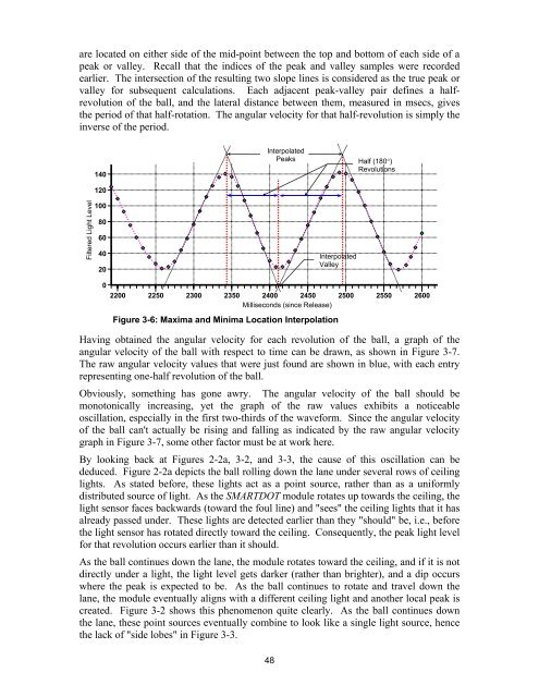
are located on either side of the mid-point between the top and bottom of each side of a
peak or valley. Recall that the indices of the peak and valley samples were recorded
earlier. The intersection of the resulting two slope lines is considered as the true peak or
valley for subsequent calculations. Each adjacent peak-valley pair defines a halfrevolution
of the ball, and the lateral distance between them, measured in msecs, gives
the period of that half-rotation. The angular velocity for that half-revolution is simply the
inverse of the period.
140
120
Interpolated
Peaks
Half (180°)
Revolutions
Filtered Light Level
100
80
60
40
20
0
2200
Interpolated
Valley
2250 2300 2350 2400 2450 2500 2550 2600
Milliseconds (since Release)
Figure 3-6: Maxima and Minima Location Interpolation
Having obtained the angular velocity for each revolution of the ball, a graph of the
angular velocity of the ball with respect to time can be drawn, as shown in Figure 3-7.
The raw angular velocity values that were just found are shown in blue, with each entry
representing one-half revolution of the ball.
Obviously, something has gone awry. The angular velocity of the ball should be
monotonically increasing, yet the graph of the raw values exhibits a noticeable
oscillation, especially in the first two-thirds of the waveform. Since the angular velocity
of the ball can't actually be rising and falling as indicated by the raw angular velocity
graph in Figure 3-7, some other factor must be at work here.
By looking back at Figures 2-2a, 3-2, and 3-3, the cause of this oscillation can be
deduced. Figure 2-2a depicts the ball rolling down the lane under several rows of ceiling
lights. As stated before, these lights act as a point source, rather than as a uniformly
distributed source of light. As the SMARTDOT module rotates up towards the ceiling, the
light sensor faces backwards (toward the foul line) and "sees" the ceiling lights that it has
already passed under. These lights are detected earlier than they "should" be, i.e., before
the light sensor has rotated directly toward the ceiling. Consequently, the peak light level
for that revolution occurs earlier than it should.
As the ball continues down the lane, the module rotates toward the ceiling, and if it is not
directly under a light, the light level gets darker (rather than brighter), and a dip occurs
where the peak is expected to be. As the ball continues to rotate and travel down the
lane, the module eventually aligns with a different ceiling light and another local peak is
created. Figure 3-2 shows this phenomenon quite clearly. As the ball continues down
the lane, these point sources eventually combine to look like a single light source, hence
the lack of "side lobes" in Figure 3-3.
48