k-Nearest Neighbor Classification on Spatial Data Streams Using P ...

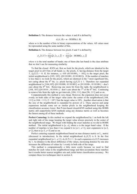
Definition 3. The distance between the values A and B is defined by
d v (A, B) = m - HOBS(A, B)
where m is the number of bits in binary representations of the values. All values must
be represented using the same number of bits.
Definition 4. The distance between two pixels X and Y is defined by
d
p
n−1
n−1
( X,Y ) = max{ d ( x ,y )} = max{ m - HOBS( x ,y )}
i=
1
v
i
i
i=
1
where n is the total number of bands; one of them (the last band) is the class attribute
that we don’t use for measuring similarity.
To find the closed –KNN set, first we look for the pixels, which are identical to the
target pixel in all 8 bits of all bands i.e. the pixels, X, having distance from the target
T, d p (X,T) = 0. If, for instance, x 1 =105 (01101001 b = 105 d ) is the target pixel, the
initial neighborhood is [105, 105] ([01101001, 01101001]). If the number of matches
is less than k, we look for the pixels, which are identical in the 7 most significant bits,
not caring about the 8 th bit, i.e. pixels having d p (X,T) ≤ 1. Therefore our expanded
neighborhood is [104,105] ([01101000, 01101001] or [0110100-, 0110100-] - don’t
care about the 8 th bit). Removing one more bit from the right, the neighborhood is
[104, 107] ([011010--, 011010--] - don’t care about the 7 th or the 8 th bit). Continuing
to remove bits from the right we get intervals, [104, 111], then [96, 111] and so on.
Computationally this method is very cheap. However, the expansion does not occur
evenly on both sides of the target value (note: the center of the neighborhood [104,
111] is (104 + 111) /2 = 107.5 but the target value is 105). Another observation is that
the size of the neighborhood is expanded by powers of 2. These uneven and jump
expansions include some not so similar pixels in the neighborhood keeping the
classification accuracy lower. But P-tree-based closed-KNN method using this HOBS
metric still outperforms KNN methods using any distance metric as well as becomes
the fastest among all of these methods.
Perfect Centering: In this method we expand the neighborhood by 1 on both the left
and right side of the range keeping the target value always precisely in the center of
the neighborhood range. We begin with finding the exact matches as we did in HOBS
method. The initial neighborhood is [a, a], where a is the target band value. If the
number of matches is less than k we expand it to [a-1, a+1], next expansion to [a-2,
a+2], then to [a-3, a+3] and so on.
Perfect centering expands neighborhood based on max distance metric or L ∞ metric
(discussed in introduction). In the initial neighborhood d ∞ (X,T) is 0. In the first
expanded neighborhood [a-1, a+1], d ∞ (X,T) ≤ 1. In each expansion d ∞ (X,T) increases
by 1. As distance is the direct difference of the values, increasing distance by one also
increases the difference of values by 1 evenly in both side of the range.
This method is computationally a little more costly because we need to find
matches for each value in the neighborhood range and then accumulate those matches
but it results better nearest neighbor sets and yields better classification accuracy. We
compare these two techniques later in section 4.
i
i