k-Nearest Neighbor Classification on Spatial Data Streams Using P ...
k-Nearest Neighbor Classification on Spatial Data Streams Using P ...
k-Nearest Neighbor Classification on Spatial Data Streams Using P ...

Create successful ePaper yourself
Turn your PDF publications into a flip-book with our unique Google optimized e-Paper software.
y<br />
B<br />
y<br />
B<br />
T<br />
A<br />
x<br />
T<br />
A<br />
x<br />
Max & Euclidian<br />
Max & Manhattan<br />
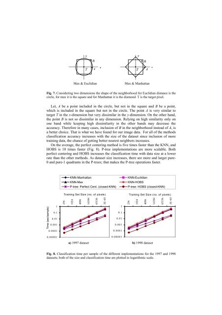
Fig. 7. C<strong>on</strong>sidering two dimensi<strong>on</strong>s the shape of the neighborhood for Euclidian distance is the<br />
circle, for max it is the square and for Manhattan it is the diam<strong>on</strong>d. T is the target pixel.<br />
Let, A be a point included in the circle, but not in the square and B be a point,<br />
which is included in the square but not in the circle. The point A is very similar to<br />
target T in the x-dimensi<strong>on</strong> but very dissimilar in the y-dimensi<strong>on</strong>. On the other hand,<br />
the point B is not so dissimilar in any dimensi<strong>on</strong>. Relying <strong>on</strong> high similarity <strong>on</strong>ly <strong>on</strong><br />
<strong>on</strong>e band while keeping high dissimilarity in the other bands may decrease the<br />
accuracy. Therefore in many cases, inclusi<strong>on</strong> of B in the neighborhood instead of A, is<br />
a better choice. That is what we have found for our image data. For all of the methods<br />
classificati<strong>on</strong> accuracy increases with the size of the dataset since inclusi<strong>on</strong> of more<br />
training data, the chance of getting better nearest neighbors increases.<br />
On the average, the perfect centering method is five times faster than the KNN, and<br />
HOBS is 10 times faster (Fig. 8). P-tree implementati<strong>on</strong>s are more scalable. Both<br />
perfect centering and HOBS increases the classificati<strong>on</strong> time with data size at a lower<br />
rate than the other methods. As dataset size increases, there are more and larger pure-<br />
0 and pure-1 quadrants in the P-trees; that makes the P-tree operati<strong>on</strong>s faster.<br />
KNN-Manhattan<br />
KNN-Max<br />
P-tree: Perfect Cent. (closed-KNN)<br />
Training Set Size (no. of pixels)<br />
KNN-Euclidian<br />
KNN-HOBS<br />
P-tree: HOBS (closed-KNN)<br />
Training Set Size (no. of pixels)<br />
Time (sec/sample)<br />
1<br />
0.1<br />
0.01<br />
0.001<br />
0.0001<br />
256<br />
1024<br />
4096<br />
16384<br />
65536<br />
3E+05<br />
1<br />
0.1<br />
0.01<br />
0.001<br />
0.0001<br />
256<br />
1024<br />
4096<br />
16384<br />
65536<br />
3E+05<br />
0.00001<br />
0.00001<br />
a) 1997 dataset b) 1998 dataset<br />
Fig. 8. <str<strong>on</strong>g>Classificati<strong>on</strong></str<strong>on</strong>g> time per sample of the different implementati<strong>on</strong>s for the 1997 and 1998<br />
datasets; both of the size and classificati<strong>on</strong> time are plotted in logarithmic scale.