k-Nearest Neighbor Classification on Spatial Data Streams Using P ...
k-Nearest Neighbor Classification on Spatial Data Streams Using P ...
k-Nearest Neighbor Classification on Spatial Data Streams Using P ...

Create successful ePaper yourself
Turn your PDF publications into a flip-book with our unique Google optimized e-Paper software.
Yield is the class attribute. Each band is 8 bits l<strong>on</strong>g. So we have 8 basic P-trees for<br />
each band and 40 (for the other 5 bands except yield) in total. For the class band, we<br />
c<strong>on</strong>sidered <strong>on</strong>ly the most significant 3 bits. Therefore we have 8 different class labels.<br />
We built 8 value P-trees from the yield values – <strong>on</strong>e for each class label.<br />
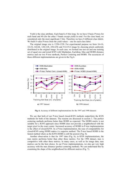
The original image size is 1320×1320. For experimental purpose we form 16×16,<br />
32×32, 64×64, 128×128, 256×256 and 512×512 image by choosing pixels uniformly<br />
distributed in the original image. In each case, we formed <strong>on</strong>e test set and <strong>on</strong>e training<br />
set of equal size and tested KNN with Manhattan, Euclidian, Max and HOBS distance<br />
metrics and our two P-tree methods, Perfect Centering and HOBS. The accuracies of<br />
these different implementati<strong>on</strong>s are given in the Fig 6.<br />
KNN-Manhattan<br />
KNN-Max<br />
P-tree: Perfect Cent. (closed-KNN)<br />
KNN-Euclidian<br />
KNN-HOBS<br />
P-tree: HOBS (closed-KNN)<br />
Accuracy (%)<br />
75<br />
70<br />
65<br />
60<br />
55<br />
50<br />
60<br />
55<br />
50<br />
45<br />
40<br />
35<br />
256<br />
1024<br />
4096<br />
16384<br />
65536<br />
3E+05<br />
Training Set Size (no. of pixels)<br />
256<br />
1024<br />
4096<br />
16384<br />
65536<br />
3E+05<br />
Training Set Size (no of pixels)<br />
a) 1997 dataset b) 1998 dataset<br />
Fig. 6. Accuracy of different implementati<strong>on</strong>s for the 1997 and 1998 datasets<br />
We see that both of our P-tree based closed-KNN methods outperform the KNN<br />
methods for both of the datasets. The reas<strong>on</strong>s are discussed in secti<strong>on</strong> 3. The perfect<br />
centering methods performs better than HOBS as expected. The HOBS metric is not<br />
suitable for a KNN approach since HOBS does not provide a neighborhood with the<br />
target pixel in the exact center. Increased accuracy of HOBS in P-tree implementati<strong>on</strong><br />
is the effect of closed-KNN. In a P-tree implementati<strong>on</strong>, the ease of computability for<br />
closed-KNN using HOBS makes it a superior method. The P-tree based HOBS is the<br />
fastest method where as the KNN-HOBS is still the poorest (Fig. 8).<br />
Another observati<strong>on</strong> is that for 1997 data (Fig. 6), in KNN implementati<strong>on</strong>s, the<br />
max metric performs better than other three metrics. For the 1998 dataset, max is<br />
competitive with other three metrics. In many cases, as well as for image data, max<br />
metrics can be the best choice. In our P-tree implementati<strong>on</strong>s, we also get very high<br />
accuracy with the max distance (perfect centering method). We can understand this by<br />
examining the shape of the neighborhood for different metrics (Fig. 7).