k-Nearest Neighbor Classification on Spatial Data Streams Using P ...
k-Nearest Neighbor Classification on Spatial Data Streams Using P ...
k-Nearest Neighbor Classification on Spatial Data Streams Using P ...

Create successful ePaper yourself
Turn your PDF publications into a flip-book with our unique Google optimized e-Paper software.
k-<str<strong>on</strong>g>Nearest</str<strong>on</strong>g> <str<strong>on</strong>g>Neighbor</str<strong>on</strong>g> <str<strong>on</strong>g>Classificati<strong>on</strong></str<strong>on</strong>g> <strong>on</strong> <strong>Spatial</strong> <strong>Data</strong><br />
<strong>Streams</strong> <strong>Using</strong> P-Trees 1, 2<br />
Maleq Khan, Qin Ding, and William Perrizo<br />
Computer Science Department, North Dakota State University<br />
Fargo, ND 58105, USA<br />
{Md.Khan, Qin.Ding, William.Perrizo}@ndsu.nodak.edu<br />
Abstract. <str<strong>on</strong>g>Classificati<strong>on</strong></str<strong>on</strong>g> of spatial data streams is crucial, since the training<br />
dataset changes often. Building a new classifier each time can be very costly<br />
with most techniques. In this situati<strong>on</strong>, k-nearest neighbor (KNN) classificati<strong>on</strong><br />
is a very good choice, since no residual classifier needs to be built ahead of<br />
time. KNN is extremely simple to implement and lends itself to a wide variety<br />
of variati<strong>on</strong>s. We propose a new method of KNN classificati<strong>on</strong> for spatial data<br />
using a new, rich, data-mining-ready structure, the Peano-count-tree (P-tree).<br />
We merely perform some AND/OR operati<strong>on</strong>s <strong>on</strong> P-trees to find the nearest<br />
neighbors of a new sample and assign the class label. We have fast and efficient<br />
algorithms for the AND/OR operati<strong>on</strong>s, which reduce the classificati<strong>on</strong> time<br />
significantly. Instead of taking exactly the k nearest neighbors we form a closed-<br />
KNN set. Our experimental results show closed-KNN yields higher<br />
classificati<strong>on</strong> accuracy as well as significantly higher speed.<br />
1. Introducti<strong>on</strong><br />
There are various techniques for classificati<strong>on</strong> such as Decisi<strong>on</strong> Tree Inducti<strong>on</strong>,<br />
Bayesian <str<strong>on</strong>g>Classificati<strong>on</strong></str<strong>on</strong>g>, and Neural Networks [7, 8]. Unlike other comm<strong>on</strong><br />
classifiers, a k-nearest neighbor (KNN) classifier does not build a classifier in<br />
advance. That is what makes it suitable for data streams. When a new sample arrives,<br />
KNN finds the k neighbors nearest to the new sample from the training space based<br />
<strong>on</strong> some suitable similarity or distance metric. The plurality class am<strong>on</strong>g the nearest<br />
neighbors is the class label of the new sample [3, 4, 5, 7]. A comm<strong>on</strong> similarity<br />
functi<strong>on</strong> is based <strong>on</strong> the Euclidian distance between two data tuples [7]. For two<br />
tuples, X = and Y = (excluding the class<br />
labels), the Euclidian similarity functi<strong>on</strong> is d ( X , Y = ( − )<br />
2 )<br />
n<br />
∑ − 1<br />
i=<br />
1<br />
x i y i<br />
2<br />
. A<br />
generalizati<strong>on</strong> of the Euclidean functi<strong>on</strong> is the Minkowski similarity functi<strong>on</strong> is<br />
1 Patents are pending <strong>on</strong> the bSQ and Ptree technology.<br />
2 This work is partially supported by NSF Grant OSR-9553368, DARPA Grant DAAH04-96-1-<br />
0329 and GSA Grant ACT#: K96130308.
n<br />
d q<br />
q X Y ∑ − 1<br />
, ) =<br />
i=<br />
1<br />
i<br />
i<br />
q<br />
i<br />
( w x − y . The Euclidean functi<strong>on</strong> results by setting q to 2 and<br />
each weight, w i , to 1. The Manhattan distance, ∑ − d 1 ( X , Y ) = x i − y i result by setting<br />
i=<br />
1<br />
q to 1. Setting q to ∞, results in the max functi<strong>on</strong> d<br />
∞<br />
n 1<br />
n<br />
= − 1<br />
max<br />
i=<br />
1<br />
( X , Y ) x − y .<br />
In this paper, we introduced a new metric called Higher Order Bit (HOB)<br />
similarity metric and evaluated the effect of all of the above distance metrics in<br />
classificati<strong>on</strong> time and accuracy. HOB distance provides an efficient way of<br />
computing neighborhoods while keeping the classificati<strong>on</strong> accuracy very high.<br />
KNN is a good choice when simplicity and accuracy are the predominant issues.<br />
KNN can be superior when a residual, trained and tested classifiers, such as ID3, has a<br />
short useful lifespan, such as in the case with data streams, where new data arrives<br />
rapidly and the training set is ever changing [1, 2]. For example, in spatial data,<br />
AVHRR images are generated in every <strong>on</strong>e hour and can be viewed as spatial data<br />
streams. The purpose of this paper is to introduce a new KNN-like model, which is<br />
not <strong>on</strong>ly simple and accurate but is also fast – fast enough for use in spatial data<br />
stream classificati<strong>on</strong>.<br />
In this paper we propose a simple and fast KNN-like classificati<strong>on</strong> algorithm for<br />
spatial data using P-trees. P-trees are new, compact, data-mining-ready data<br />
structures, which provide a lossless representati<strong>on</strong> of the original spatial data [6, 9,<br />
10]. In the secti<strong>on</strong> 2, we review the structure of P-trees and various P-tree operati<strong>on</strong>s.<br />
We c<strong>on</strong>sider a space to be represented by a 2-dimensi<strong>on</strong>al array of locati<strong>on</strong>s.<br />
Associated with each locati<strong>on</strong> are various attributes, called bands, such as visible<br />
reflectance intensities (blue, green and red), infrared reflectance intensities (e.g., NIR,<br />
MIR1, MIR2 and TIR) and possibly crop yield quantities, soil attributes and radar<br />
reflectance intensities. We refer to a locati<strong>on</strong> as a pixel in this paper.<br />
<strong>Using</strong> P-trees, we presented two algorithms, <strong>on</strong>e based <strong>on</strong> the max distance metric<br />
and the other based <strong>on</strong> our new HOB distance metric. HOB is the similarity of the<br />
most significant bit positi<strong>on</strong>s in each band. It differs from pure Euclidean similarity<br />
in that it can be an asymmetric functi<strong>on</strong> depending up<strong>on</strong> the bit arrangement of the<br />
values involved. However, it is very fast, very simple and quite accurate. Instead of<br />
using exactly k nearest neighbor (a KNN set), our algorithms build a closed-KNN set<br />
and perform voting <strong>on</strong> this closed-KNN set to find the predicting class. Closed-KNN,<br />
a superset of KNN, is formed by including the pixels, which have the same distance<br />
from the target pixel as some of the pixels in KNN set. Based <strong>on</strong> this similarity<br />
measure, finding nearest neighbors of new samples (pixel to be classified) can be<br />
d<strong>on</strong>e easily and very efficiently using P-trees and we found higher classificati<strong>on</strong><br />
accuracy than traditi<strong>on</strong>al methods <strong>on</strong> c<strong>on</strong>sidered datasets. Detailed definiti<strong>on</strong>s of the<br />
similarity and the algorithms to find nearest neighbors are given in the secti<strong>on</strong> 3. We<br />
provided experimental results and analyses in secti<strong>on</strong> 4. The c<strong>on</strong>clusi<strong>on</strong> is given in<br />
Secti<strong>on</strong> 5.<br />
i<br />
i
2. P-tree <strong>Data</strong> Structures<br />
Most spatial data comes in a format called BSQ for Band Sequential (or can be easily<br />
c<strong>on</strong>verted to BSQ). BSQ data has a separate file for each band. The ordering of the<br />
data values within a band is raster ordering with respect to the spatial area represented<br />
in the dataset. We divided each BSQ band into several files, <strong>on</strong>e for each bit positi<strong>on</strong><br />
of the data values. We call this format bit Sequential or bSQ [6, 9, 10]. A Landsat<br />
Thematic Mapper satellite image, for example, is in BSQ format with 7 bands,<br />
B 1 ,…,B 7 , (Landsat-7 has 8) and ~40,000,000 8-bit data values. A typical TIFF image<br />
aerial digital photograph is <strong>on</strong>e file c<strong>on</strong>taining ~24,000,000 bits ordered by itpositi<strong>on</strong>,<br />
then band and then raster-ordered-pixel-locati<strong>on</strong>.<br />
We organize each bSQ bit file, B ij (the file c<strong>on</strong>structed from the j th bits of i th band),<br />
into a tree structure, called a Peano Count Tree (P-tree). A P-tree is a quadrant-based<br />
tree. The root of a P-tree c<strong>on</strong>tains the 1-bit count, called root count, of the entire bitband.<br />
The next level of the tree c<strong>on</strong>tains the 1-bit counts of the four quadrants in<br />
raster order. At the next level, each quadrant is partiti<strong>on</strong>ed into sub-quadrants and<br />
their 1-bit counts in raster order c<strong>on</strong>stitute the children of the quadrant node. This<br />
c<strong>on</strong>structi<strong>on</strong> is c<strong>on</strong>tinued recursively down each tree path until the sub-quadrant is<br />
pure (entirely 1-bits or entirely 0-bits). Recursive raster ordering is called the Peano<br />
or Z-ordering in the literature – therefore, the name Peano Count trees. The P-tree for<br />
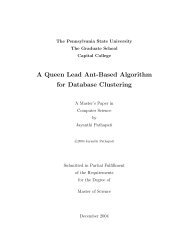
a 8-row-8-column bit-band is shown in Fig. 1.<br />
1 1 1 1 1 1 0 0<br />
1 1 1 1 1 0 0 0<br />
1 1 1 1 1 1 0 0<br />
1 1 1 1 1 1 1 0<br />
1 1 1 1 1 1 1 1<br />
1 1 1 1 1 1 1 1<br />
1 1 1 1 1 1 1 1<br />
0 1 1 1 1 1 1 1<br />
55<br />
____________/ / \ \_________<br />
/ _____/ \ ___ \<br />
16 ____8__ _15__ 16<br />
/ / | \ / | \ \<br />
3 0 4 1 4 4 3 4<br />
//|\ //|\ //|\<br />
1110 0010 1101<br />
m<br />
_____________/ / \ \_________<br />
/ ____/ \ ____ \<br />
1 ____m__ _m__ 1<br />
/ / | \ / | \ \<br />
m 0 1 m 1 1 m 1<br />
//|\ //|\ //|\<br />
1110 0010 1101<br />
Fig. 1. 8-by-8 image and its P-tree (P-tree and PM-tree)<br />
In this example, root count is 55, and the counts at the next level, 16, 8, 15 and 16,<br />
are the 1-bit counts for the four major quadrants. Since the first and last quadrant is<br />
made up of entirely 1-bits, we do not need sub-trees for these two quadrants.<br />
For each band (assuming 8-bit data values), we get 8 basic P-trees. P i,j is the P-tree<br />
for the j th bits of the values from the i th band. For efficient implementati<strong>on</strong>, we use<br />
variati<strong>on</strong> of basic P-trees, called Pure Mask tree (PM-tree). In the PM-tree, we use a<br />
3-value logic, in which 11 represents a quadrant of pure 1-bits, pure1 quadrant, 00<br />
represents a quadrant of pure 0-bits, pure0 quadrant, and 01 represents a mixed<br />
quadrant. To simplify the expositi<strong>on</strong>, we use 1 instead of 11 for pure1, 0 for pure0,<br />
and m for mixed. The PM-tree for the previous example is also given in Fig. 1.<br />
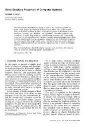
P-tree algebra c<strong>on</strong>tains operators, AND, OR, NOT and XOR, which are the pixelby-pixel<br />
logical operati<strong>on</strong>s <strong>on</strong> P-trees. The AND/OR operati<strong>on</strong>s <strong>on</strong> PM-trees are<br />
shown in Fig. 2. The AND operati<strong>on</strong> between two PM-trees is performed by ANDing
the corresp<strong>on</strong>ding nodes in the two operand PM-trees level-by-level starting from the<br />
root node. A pure0 node ANDed with any node produces a pure0 node. A pure1 node<br />
ANDed with any node, n, produces the node n; we just need to copy the node, n, to<br />
the resultant PM-tree in the corresp<strong>on</strong>ding positi<strong>on</strong>. ANDing of two mixed nodes<br />
produces a mixed node; the children of the resultant mixed node are obtained by<br />
ANDing children of the operands recursively. The details of P-tree operati<strong>on</strong>s can be<br />
found in [10, 11].<br />
P-tree-1: m<br />
____/ / \ \____<br />
/ / \ \<br />
/ / \ \<br />
1 m m 1<br />
/ / \ \ / / \ \<br />
m 0 1 m 1 1 m 1<br />
//|\ //|\ //|\<br />
1110 0010 1101<br />
P-tree-2: m<br />
____/ / \ \____<br />
/ / \ \<br />
/ / \ \<br />
1 0 m 0<br />
/ / \ \<br />
1 1 1 m<br />
//|\<br />
0100<br />
AND: m<br />
___ / / \ \___<br />
/ ___ / \ \<br />
/ / \ \<br />
1 0 m 0<br />
/ | \ \<br />
1 1 m m<br />
//|\ //|\<br />
1101 0100<br />
OR: m<br />
___ / / \ \__<br />
/ __ / \ \<br />
/ / \ \<br />
1 m 1 1<br />
/ / \ \<br />
m 0 1 m<br />
//|\ //|\<br />
1110 0010<br />
Fig. 2. P-tree Algebra<br />
3. The <str<strong>on</strong>g>Classificati<strong>on</strong></str<strong>on</strong>g> Algorithms<br />
In the original k-nearest neighbor (KNN) classificati<strong>on</strong> method, no classifier model is<br />
built in advance. KNN refers back to the raw training data in the classificati<strong>on</strong> of each<br />
new sample. Therefore, <strong>on</strong>e can say that the entire training set is the classifier. The<br />
basic idea is that the similar tuples most likely bel<strong>on</strong>gs to the same class (a c<strong>on</strong>tinuity<br />
assumpti<strong>on</strong>). Based <strong>on</strong> some pre-selected distance metric (some comm<strong>on</strong>ly used<br />
distance metrics are discussed in introducti<strong>on</strong>), it finds the k most similar or nearest<br />
training samples of the sample to be classified and assign the plurality class of those k<br />
samples to the new sample [4, 7]. The value for k is pre-selected. <strong>Using</strong> relatively<br />
larger k may include some not so similar pixels and <strong>on</strong> the other hand, using very<br />
smaller k may exclude some potential candidate pixels. In both cases the classificati<strong>on</strong><br />
accuracy will decrease. The optimal value of k depends <strong>on</strong> the size and nature of the<br />
data. The typical value for k is 3, 5 or 7. The steps of the classificati<strong>on</strong> process are:<br />
1) Determine a suitable distance metric.<br />
2) Find the k nearest neighbors using the selected distance metric.<br />
3) Find the plurality class of the k-nearest neighbors (voting <strong>on</strong> the class<br />
labels of the NNs).<br />
4) Assign that class to the sample to be classified.<br />
We provided two different algorithms using P-trees, based two different distance<br />
metrics max (Minkowski distance with q = ∞) and our newly defined HOB distance.<br />
Instead of examining individual pixels to find the nearest neighbors, we start our<br />
initial neighborhood (neighborhood is a set of neighbors of the target pixel within a<br />
specified distance based <strong>on</strong> some distance metric, not the spatial neighbors, neighbors<br />
with respect to values) with the target sample and then successively expand the
neighborhood area until there are k pixels in the neighborhood set. The expansi<strong>on</strong> is<br />
d<strong>on</strong>e in such a way that the neighborhood always c<strong>on</strong>tains the closest or most similar<br />
pixels of the target sample. The different expansi<strong>on</strong> mechanisms implement different<br />
distance functi<strong>on</strong>s. In the next secti<strong>on</strong> (secti<strong>on</strong> 3.1) we described the distance metrics<br />
and expansi<strong>on</strong> mechanisms.<br />
Of course, there may be more boundary neighbors equidistant from the sample than<br />
are necessary to complete the k nearest neighbor set, in which case, <strong>on</strong>e can either use<br />
the larger set or arbitrarily ignore some of them. To find the exact k nearest neighbors<br />
<strong>on</strong>e has to arbitrarily ignore some of them.<br />
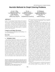
T<br />
Fig. 3. T, the pixel in the center is the target pixels. With k = 3, to find the third nearest<br />
neighbor, we have four pixels (<strong>on</strong> the boundary line of the neighborhood) which are equidistant<br />
from the target.<br />
Instead we propose a new approach of building nearest neighbor (NN) set, where<br />
we take the closure of the k-NN set, that is, we include all of the boundary neighbors<br />
and we call it the closed-KNN set. Obviously closed-KNN is a superset of KNN set. In<br />
the above example, with k = 3, KNN includes the two points inside the circle and any<br />
<strong>on</strong>e point <strong>on</strong> the boundary. The closed-KNN includes the two points in side the circle<br />
and all of the four boundary points. The inductive definiti<strong>on</strong> of the closed-KNN set is<br />
given below.<br />
Definiti<strong>on</strong> 1. a) If x ∈ KNN, then x ∈ closed-KNN<br />
b) If x ∈ closed-KNN and d(T,y) ≤ d(T,x), then y ∈ closed-KNN<br />
where, d(T,x) is the distance of x from target T.<br />
c) Closed-KNN does not c<strong>on</strong>tain any pixel, which cannot be produced<br />
by steps a and b.<br />
Our experimental results show closed-KNN yields higher classificati<strong>on</strong> accuracy<br />
than KNN does. The reas<strong>on</strong> is if for some target there are many pixels <strong>on</strong> the<br />
boundary, they have more influence <strong>on</strong> the target pixel. While all of them are in the<br />
nearest neighborhood area, inclusi<strong>on</strong> of <strong>on</strong>e or two of them does not provide the<br />
necessary weight in the voting mechanism. One may argue that then why d<strong>on</strong>’t we use<br />
a higher k? For example using k = 5 instead of k = 3. The answer is if there are too<br />
few points (for example <strong>on</strong>ly <strong>on</strong>e or two points) <strong>on</strong> the boundary to make k neighbors<br />
in the neighborhood, we have to expand neighborhood and include some not so<br />
similar points which will decrease the classificati<strong>on</strong> accuracy. We c<strong>on</strong>struct closed-<br />
KNN <strong>on</strong>ly by including those pixels, which are in as same distance as some other<br />
pixels in the neighborhood without further expanding the neighborhood. To perform
our experiments, we find the optimal k (by trial and error method) for that particular<br />
dataset and then using the optimal k, we performed both KNN and closed-KNN and<br />
found higher accuracy for P-tree-based closed-KNN method. The experimental results<br />
are given in secti<strong>on</strong> 4. In our P-tree implementati<strong>on</strong>, no extra computati<strong>on</strong> is required<br />
to find the closed-KNN. Our expansi<strong>on</strong> mechanism of nearest neighborhood<br />
automatically includes the points <strong>on</strong> the boundary of the neighborhood.<br />
Also, there may be more than <strong>on</strong>e class in plurality (if there is a tie in voting), in<br />
which case <strong>on</strong>e can arbitrarily chose <strong>on</strong>e of the plurality classes. Without storing the<br />
raw data we create the basic P-trees and store them for future classificati<strong>on</strong> purpose.<br />
Avoiding the examinati<strong>on</strong> of individual data points and being ready for data mining<br />
these P-trees not <strong>on</strong>ly saves classificati<strong>on</strong> time but also saves storage space, since data<br />
is stored in compressed form. This compressi<strong>on</strong> technique also increases the speed of<br />
ANDing and other operati<strong>on</strong>s <strong>on</strong> P-trees, since operati<strong>on</strong>s can be performed <strong>on</strong> the<br />
pure0 and pure1 quadrants without reference to individual bits, since all of the bits in<br />
those quadrants are the same.<br />
3.1 Expansi<strong>on</strong> of <str<strong>on</strong>g>Neighbor</str<strong>on</strong>g>hood and Distance or Similarity Metrics<br />
We begin searching for nearest neighbors by finding the exact matches. If the number<br />
of exact matches is less than k, we expand the neighborhood. The expansi<strong>on</strong> of the<br />
neighborhood in each dimensi<strong>on</strong> are d<strong>on</strong>e simultaneously, and c<strong>on</strong>tinued until the<br />
number pixels in the neighborhood is greater than or equal to k. We develop the<br />
following two different mechanisms, corresp<strong>on</strong>ding to max distance and our newly<br />
defined HOB distance, for expanding the neighborhood. They have trade offs between<br />
executi<strong>on</strong> time and classificati<strong>on</strong> accuracy.<br />
Higher Order Bit Similarity (HOBS): We propose a new similarity metric where<br />
we c<strong>on</strong>sider similarity in the most significant c<strong>on</strong>secutive bit positi<strong>on</strong>s starting from<br />
the left most bit, the highest order bit. C<strong>on</strong>sider the following two values, x 1 and y 1,<br />
represented in binary. The 1 st bit is the most significant bit and 8 th bit is the least<br />
significant bit.<br />
Bit positi<strong>on</strong>: 1 2 3 4 5 6 7 8 1 2 3 4 5 6 7 8<br />
x 1 : 0 1 1 0 1 0 0 1 x 1 : 0 1 1 0 1 0 0 1<br />
y 1 : 0 1 1 1 1 1 0 1 y 2 : 0 1 1 0 0 1 0 0<br />
These two values are similar in the three most significant bit positi<strong>on</strong>s, 1 st , 2 nd and<br />
3 rd bits (011). After they differ (4 th bit), we d<strong>on</strong>’t c<strong>on</strong>sider anymore lower order bit<br />
positi<strong>on</strong>s though x 1 and y 1 have identical bits in the 5 th , 7 th and 8 th positi<strong>on</strong>s. Since we<br />
are looking for closeness in values, after differing in some higher order bit positi<strong>on</strong>s,<br />
similarity in some lower order bit is meaningless with respect to our purpose.<br />
Similarly, x 1 and y 2 are identical in the 4 most significant bits (0110). Therefore,<br />
according to our definiti<strong>on</strong>, x 1 is closer or similar to y 2 than to y 1 .<br />
Definiti<strong>on</strong> 2. The similarity between two integers A and B is defined by<br />
HOBS(A, B) = max{s | 0 ≤ i ≤ s ⇒ a i = b i }<br />
in other words, HOBS(A, B) = s, where for all i ≤ s and 0 ≤ i, a i = b i and a s+1 ≠ b s+1 .<br />
a i and b i are the i th bits of A and B respectively.
Definiti<strong>on</strong> 3. The distance between the values A and B is defined by<br />
d v (A, B) = m - HOBS(A, B)<br />
where m is the number of bits in binary representati<strong>on</strong>s of the values. All values must<br />
be represented using the same number of bits.<br />
Definiti<strong>on</strong> 4. The distance between two pixels X and Y is defined by<br />
d<br />
p<br />
n−1<br />
n−1<br />
( X,Y ) = max{ d ( x ,y )} = max{ m - HOBS( x ,y )}<br />
i=<br />
1<br />
v<br />
i<br />
i<br />
i=<br />
1<br />
where n is the total number of bands; <strong>on</strong>e of them (the last band) is the class attribute<br />
that we d<strong>on</strong>’t use for measuring similarity.<br />
To find the closed –KNN set, first we look for the pixels, which are identical to the<br />
target pixel in all 8 bits of all bands i.e. the pixels, X, having distance from the target<br />
T, d p (X,T) = 0. If, for instance, x 1 =105 (01101001 b = 105 d ) is the target pixel, the<br />
initial neighborhood is [105, 105] ([01101001, 01101001]). If the number of matches<br />
is less than k, we look for the pixels, which are identical in the 7 most significant bits,<br />
not caring about the 8 th bit, i.e. pixels having d p (X,T) ≤ 1. Therefore our expanded<br />
neighborhood is [104,105] ([01101000, 01101001] or [0110100-, 0110100-] - d<strong>on</strong>’t<br />
care about the 8 th bit). Removing <strong>on</strong>e more bit from the right, the neighborhood is<br />
[104, 107] ([011010--, 011010--] - d<strong>on</strong>’t care about the 7 th or the 8 th bit). C<strong>on</strong>tinuing<br />
to remove bits from the right we get intervals, [104, 111], then [96, 111] and so <strong>on</strong>.<br />
Computati<strong>on</strong>ally this method is very cheap. However, the expansi<strong>on</strong> does not occur<br />
evenly <strong>on</strong> both sides of the target value (note: the center of the neighborhood [104,<br />
111] is (104 + 111) /2 = 107.5 but the target value is 105). Another observati<strong>on</strong> is that<br />
the size of the neighborhood is expanded by powers of 2. These uneven and jump<br />
expansi<strong>on</strong>s include some not so similar pixels in the neighborhood keeping the<br />
classificati<strong>on</strong> accuracy lower. But P-tree-based closed-KNN method using this HOBS<br />
metric still outperforms KNN methods using any distance metric as well as becomes<br />
the fastest am<strong>on</strong>g all of these methods.<br />
Perfect Centering: In this method we expand the neighborhood by 1 <strong>on</strong> both the left<br />
and right side of the range keeping the target value always precisely in the center of<br />
the neighborhood range. We begin with finding the exact matches as we did in HOBS<br />
method. The initial neighborhood is [a, a], where a is the target band value. If the<br />
number of matches is less than k we expand it to [a-1, a+1], next expansi<strong>on</strong> to [a-2,<br />
a+2], then to [a-3, a+3] and so <strong>on</strong>.<br />
Perfect centering expands neighborhood based <strong>on</strong> max distance metric or L ∞ metric<br />
(discussed in introducti<strong>on</strong>). In the initial neighborhood d ∞ (X,T) is 0. In the first<br />
expanded neighborhood [a-1, a+1], d ∞ (X,T) ≤ 1. In each expansi<strong>on</strong> d ∞ (X,T) increases<br />
by 1. As distance is the direct difference of the values, increasing distance by <strong>on</strong>e also<br />
increases the difference of values by 1 evenly in both side of the range.<br />
This method is computati<strong>on</strong>ally a little more costly because we need to find<br />
matches for each value in the neighborhood range and then accumulate those matches<br />
but it results better nearest neighbor sets and yields better classificati<strong>on</strong> accuracy. We<br />
compare these two techniques later in secti<strong>on</strong> 4.<br />
i<br />
i
3.2 Computing the <str<strong>on</strong>g>Nearest</str<strong>on</strong>g> <str<strong>on</strong>g>Neighbor</str<strong>on</strong>g>s<br />
For HOBS: P i,j is the basic P-tree for bit j of band i and P′ i,j is the complement of P i,j .<br />
Let, b i,j = j th bit of the i th band of the target pixel, and define<br />
Pt i,j = P i,j , if b i,j = 1,<br />
= P′ i,j , otherwise.<br />
We can say that the root count of Pt i,j is the number of pixels in the training dataset<br />
having as same value as the j th bit of the i th band of the target pixel. Let,<br />
Pv i,1-j = Pt i,1 & Pt i,2 & Pt i,3 & … & Pt i,j , and<br />
Pd(j) = Pv 1,1-j & Pv 2,1- j & Pv 3,1- j & … & Pv n-1,1- j<br />
where & is the P-tree AND operator and n is the number of bands. Pv i,1-j counts the<br />
pixels having as same bit values as the target pixel in the higher order j bits of i th<br />
band. We calculate the initial neighborhood P-tree, Pnn = Pd(8), the exact matching,<br />
c<strong>on</strong>sidering 8-bit values. Then we calculate Pnn = Pd(7), matching in 7 higher order<br />
bits; then Then Pnn = Pd(6) and so <strong>on</strong>. We c<strong>on</strong>tinue as l<strong>on</strong>g as root count of Pnn is<br />
less than k. Pnn represents closed-KNN set and the root count of Pnn is the number of<br />
the nearest pixels. A 1 bit in Pnn for a pixel means that pixel is in closed-KNN set.<br />
The algorithm for finding nearest neighbors is given in Fig. 4.<br />
Input: P i,j for all bit i and band j, the basic P-trees<br />
and b i,j for all i and j, the bits for the target pixels<br />
Output: Pnn, the P-tree representing closed-KNN<br />
// n - # of bands, m - # of bits in each band<br />
FOR i = 1 TO n-1 D<br />
FOR j = 1 TO m DO<br />
IF b i,j = 1 Pt ij P i,j<br />
ELSE Pt i,j P′ i,j<br />
FOR i = 1 TO n-1 DO<br />
Pv i,1 Pt i,1<br />
FOR j = 2 TO m DO<br />
Pv i,j Pv i,j-1 & Pt i,j<br />
s m<br />
REPEAT<br />
Pnn Pv 1,s<br />
FOR r = 2 TO n-1 DO<br />
Pnn Pnn & Pv r,s<br />
s s - 1<br />
UNTIL RootCount(Pnn) ≥ k<br />
Fig. 4. Algorithm to find closed-KNN set based <strong>on</strong> HOB metric<br />
For Perfect Centering: Let v i is the value of the target pixels for band i. The value P-<br />
tree, P i (v i ), represents the pixels having value v i in band i. The algorithm for<br />
computing the value P-trees is given in Fig. 5(b). For finding the initial nearest<br />
neighbors (the exact matches), we calculate<br />
Pnn = P 1 (v 1 ) & P 2 (v 2 ) & P 3 (v 3 ) & … & P n-1 (v n-1 )<br />
that represents the pixels having the same values in each band as that of the target<br />
pixel. If the root count of Pnn ≤ k, we expand neighborhood al<strong>on</strong>g each dimensi<strong>on</strong>.<br />
For each band i, we calculate range P-tree Pr i = P i (v i -1) | P i (v i ) | P i (v i +1). ‘|’ is the P-<br />
tree OR operator. Pr i represents the pixels having any value in the range [v i -1, v i +1] of<br />
band i. The ANDed result of these range P-trees, Pr i , for all i, produce the expanded<br />
neighborhood. The algorithm is given in Fig. 5(a).
Input: P i,j for all i and j, basic P-trees and<br />
v i for all i, band values of target pixel<br />
Output: Pnn, closed-KNN P-tree<br />
// n - # of bands, m- #of bits in each band<br />
FOR i = 1 TO n-1 DO<br />
Pr i P i (v i )<br />
Pnn Pr 1<br />
FOR i = 2 TO n-1 DO<br />
Pnn Pnn & Pr i //initial neighborhood<br />
d 1 // distance for the first expansi<strong>on</strong><br />
WHILE RootCount(Pnn) < k DO<br />
FOR i = 1 to n-1 DO // expansi<strong>on</strong><br />
Pr i Pr i | P i (v i -d) | P i (v i +d)<br />
Pnn Pr 1 // ‘|’ - OR operator<br />
FOR i = 2 TO n-1 DO<br />
Pnn Pnn AND Pr i<br />
d d + 1<br />
Input: P i,j for all j, basic P-trees of all<br />
the bits of band i and the value v i for<br />
band i.<br />
Output: P i (v i ), the value p-tree for the<br />
value v i<br />
// m is the number of bits in each band<br />
// b i , j is the j th bit of value v i<br />
FOR j = 1 TO m DO<br />
IF b i,j = 1 Pt ij P i,j<br />
ELSE Pt i,j P′ i,j<br />
P i (v) Pt i,1<br />
FOR j = 2 TO m DO<br />
P i (v) P i (v) & Pt i,j<br />
Fig. 5(a). Algorithm to find closed-KNN set<br />
based <strong>on</strong> Max metric (Perfect Centering).<br />
5(b). Algorithm to compute value P-trees<br />
3.3 Finding the plurality class am<strong>on</strong>g the nearest neighbors<br />
For the classificati<strong>on</strong> purpose, we d<strong>on</strong>’t need to c<strong>on</strong>sider all bits in the class band.<br />
If the class band is 8 bits l<strong>on</strong>g, there are 256 possible classes. Instead, we partiti<strong>on</strong> the<br />
class band values into fewer, say 8, groups by truncating the 5 least significant bits.<br />
The 8 classes are 0, 1, 2, …, 7. <strong>Using</strong> the leftmost 3 bits we c<strong>on</strong>struct the value P-trees<br />
P n (0), P n (1), …, P n (7). The P-tree Pnn & P n (i) represents the pixels having a class<br />
value i and are in the closed-KNN set, Pnn. An i which yields the maximum root<br />
count of Pnn & P n (i) is the plurality class; that is<br />
predicted class = arg max{ RootCount( Pnn & P () i )}.<br />
i<br />
n<br />
4. Performance Analysis<br />
We performed experiments <strong>on</strong> two sets of Arial photographs of the Best Management<br />
Plot (BMP) of Oakes Irrigati<strong>on</strong> Test Area (OITA) near Oaks, North Dakota, United<br />
States. The latitude and l<strong>on</strong>gitude are 45°49’15”N and 97°42’18”W respectively. The<br />
two images “29NW083097.tiff” and “29NW082598.tiff” have been taken in 1997 and<br />
1998 respectively. Each image c<strong>on</strong>tains 3 bands, red, green and blue reflectance<br />
values. Three other separate files c<strong>on</strong>tain synchr<strong>on</strong>ized soil moisture, nitrate and yield<br />
values. Soil moisture and nitrate are measured using shallow and deep well<br />
lysimeters. Yield values were collected by using a GPS yield m<strong>on</strong>itor <strong>on</strong> the<br />
harvesting equipments. The datasets are available at http://datasurg.ndsu.edu/.
Yield is the class attribute. Each band is 8 bits l<strong>on</strong>g. So we have 8 basic P-trees for<br />
each band and 40 (for the other 5 bands except yield) in total. For the class band, we<br />
c<strong>on</strong>sidered <strong>on</strong>ly the most significant 3 bits. Therefore we have 8 different class labels.<br />
We built 8 value P-trees from the yield values – <strong>on</strong>e for each class label.<br />
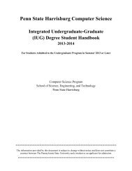
The original image size is 1320×1320. For experimental purpose we form 16×16,<br />
32×32, 64×64, 128×128, 256×256 and 512×512 image by choosing pixels uniformly<br />
distributed in the original image. In each case, we formed <strong>on</strong>e test set and <strong>on</strong>e training<br />
set of equal size and tested KNN with Manhattan, Euclidian, Max and HOBS distance<br />
metrics and our two P-tree methods, Perfect Centering and HOBS. The accuracies of<br />
these different implementati<strong>on</strong>s are given in the Fig 6.<br />
KNN-Manhattan<br />
KNN-Max<br />
P-tree: Perfect Cent. (closed-KNN)<br />
KNN-Euclidian<br />
KNN-HOBS<br />
P-tree: HOBS (closed-KNN)<br />
Accuracy (%)<br />
75<br />
70<br />
65<br />
60<br />
55<br />
50<br />
60<br />
55<br />
50<br />
45<br />
40<br />
35<br />
256<br />
1024<br />
4096<br />
16384<br />
65536<br />
3E+05<br />
Training Set Size (no. of pixels)<br />
256<br />
1024<br />
4096<br />
16384<br />
65536<br />
3E+05<br />
Training Set Size (no of pixels)<br />
a) 1997 dataset b) 1998 dataset<br />
Fig. 6. Accuracy of different implementati<strong>on</strong>s for the 1997 and 1998 datasets<br />
We see that both of our P-tree based closed-KNN methods outperform the KNN<br />
methods for both of the datasets. The reas<strong>on</strong>s are discussed in secti<strong>on</strong> 3. The perfect<br />
centering methods performs better than HOBS as expected. The HOBS metric is not<br />
suitable for a KNN approach since HOBS does not provide a neighborhood with the<br />
target pixel in the exact center. Increased accuracy of HOBS in P-tree implementati<strong>on</strong><br />
is the effect of closed-KNN. In a P-tree implementati<strong>on</strong>, the ease of computability for<br />
closed-KNN using HOBS makes it a superior method. The P-tree based HOBS is the<br />
fastest method where as the KNN-HOBS is still the poorest (Fig. 8).<br />
Another observati<strong>on</strong> is that for 1997 data (Fig. 6), in KNN implementati<strong>on</strong>s, the<br />
max metric performs better than other three metrics. For the 1998 dataset, max is<br />
competitive with other three metrics. In many cases, as well as for image data, max<br />
metrics can be the best choice. In our P-tree implementati<strong>on</strong>s, we also get very high<br />
accuracy with the max distance (perfect centering method). We can understand this by<br />
examining the shape of the neighborhood for different metrics (Fig. 7).
y<br />
B<br />
y<br />
B<br />
T<br />
A<br />
x<br />
T<br />
A<br />
x<br />
Max & Euclidian<br />
Max & Manhattan<br />
Fig. 7. C<strong>on</strong>sidering two dimensi<strong>on</strong>s the shape of the neighborhood for Euclidian distance is the<br />
circle, for max it is the square and for Manhattan it is the diam<strong>on</strong>d. T is the target pixel.<br />
Let, A be a point included in the circle, but not in the square and B be a point,<br />
which is included in the square but not in the circle. The point A is very similar to<br />
target T in the x-dimensi<strong>on</strong> but very dissimilar in the y-dimensi<strong>on</strong>. On the other hand,<br />
the point B is not so dissimilar in any dimensi<strong>on</strong>. Relying <strong>on</strong> high similarity <strong>on</strong>ly <strong>on</strong><br />
<strong>on</strong>e band while keeping high dissimilarity in the other bands may decrease the<br />
accuracy. Therefore in many cases, inclusi<strong>on</strong> of B in the neighborhood instead of A, is<br />
a better choice. That is what we have found for our image data. For all of the methods<br />
classificati<strong>on</strong> accuracy increases with the size of the dataset since inclusi<strong>on</strong> of more<br />
training data, the chance of getting better nearest neighbors increases.<br />
On the average, the perfect centering method is five times faster than the KNN, and<br />
HOBS is 10 times faster (Fig. 8). P-tree implementati<strong>on</strong>s are more scalable. Both<br />
perfect centering and HOBS increases the classificati<strong>on</strong> time with data size at a lower<br />
rate than the other methods. As dataset size increases, there are more and larger pure-<br />
0 and pure-1 quadrants in the P-trees; that makes the P-tree operati<strong>on</strong>s faster.<br />
KNN-Manhattan<br />
KNN-Max<br />
P-tree: Perfect Cent. (closed-KNN)<br />
Training Set Size (no. of pixels)<br />
KNN-Euclidian<br />
KNN-HOBS<br />
P-tree: HOBS (closed-KNN)<br />
Training Set Size (no. of pixels)<br />
Time (sec/sample)<br />
1<br />
0.1<br />
0.01<br />
0.001<br />
0.0001<br />
256<br />
1024<br />
4096<br />
16384<br />
65536<br />
3E+05<br />
1<br />
0.1<br />
0.01<br />
0.001<br />
0.0001<br />
256<br />
1024<br />
4096<br />
16384<br />
65536<br />
3E+05<br />
0.00001<br />
0.00001<br />
a) 1997 dataset b) 1998 dataset<br />
Fig. 8. <str<strong>on</strong>g>Classificati<strong>on</strong></str<strong>on</strong>g> time per sample of the different implementati<strong>on</strong>s for the 1997 and 1998<br />
datasets; both of the size and classificati<strong>on</strong> time are plotted in logarithmic scale.
5. C<strong>on</strong>clusi<strong>on</strong><br />
In this paper we proposed a new approach to k-nearest neighbor classificati<strong>on</strong> for<br />
spatial data streams by using a new data structure called the P-tree, which is a lossless<br />
compressed and data-mining-ready representati<strong>on</strong> of the original spatial data. Our new<br />
approach, called closed-KNN, finds the closure of the KNN set, we call the closed-<br />
KNN, instead of c<strong>on</strong>sidering exactly k nearest neighbors. Closed-KNN includes all of<br />
the points <strong>on</strong> the boundary even if the size of the nearest neighbor set becomes larger<br />
than k. Instead of examining individual data points to find nearest neighbors, we rely<br />
<strong>on</strong> the expansi<strong>on</strong> of the neighborhood. The P-tree structure facilitates efficient<br />
computati<strong>on</strong> of the nearest neighbors. Our methods outperform the traditi<strong>on</strong>al<br />
implementati<strong>on</strong>s of KNN both in terms of accuracy and speed.<br />
We proposed a new distance metric called Higher Order Bit (HOB) distance that<br />
provides an easy and efficient way of computing closed-KNN using P-trees while<br />
preserving the classificati<strong>on</strong> accuracy at a high level.<br />
References<br />
1. Domingos, P. and Hulten, G., “Mining high-speed data streams”, Proceedings of ACM<br />
SIGKDD 2000.<br />
2. Domingos, P., & Hulten, G., “Catching Up with the <strong>Data</strong>: Research Issues in Mining <strong>Data</strong><br />
<strong>Streams</strong>”, DMKD 2001.<br />
3. T. Cover and P. Hart, “<str<strong>on</strong>g>Nearest</str<strong>on</strong>g> <str<strong>on</strong>g>Neighbor</str<strong>on</strong>g> pattern classificati<strong>on</strong>”, IEEE Trans. Informati<strong>on</strong><br />
Theory, 13:21-27, 1967.<br />
4. Dasarathy, B.V., “<str<strong>on</strong>g>Nearest</str<strong>on</strong>g>-<str<strong>on</strong>g>Neighbor</str<strong>on</strong>g> <str<strong>on</strong>g>Classificati<strong>on</strong></str<strong>on</strong>g> Techniques”. IEEE Computer Society<br />
Press, Los Alomitos, CA, 1991.<br />
5. Morin, R.L. and D.E.Raeside, “A Reappraisal of Distance-Weighted k-<str<strong>on</strong>g>Nearest</str<strong>on</strong>g> <str<strong>on</strong>g>Neighbor</str<strong>on</strong>g><br />
<str<strong>on</strong>g>Classificati<strong>on</strong></str<strong>on</strong>g> for Pattern Recogniti<strong>on</strong> with Missing <strong>Data</strong>”, IEEE Transacti<strong>on</strong>s <strong>on</strong> Systems,<br />
Man, and Cybernetics, Vol. SMC-11 (3), pp. 241-243, 1981.<br />
6. William Perrizo, "Peano Count Tree Technology", Technical Report NDSU-CSOR-TR-<br />
01-1, 2001.<br />
7. Jiawei Han, Micheline Kamber, “<strong>Data</strong> Mining: C<strong>on</strong>cepts and Techniques”, Morgan<br />
Kaufmann, 2001.<br />
8. M. James, “<str<strong>on</strong>g>Classificati<strong>on</strong></str<strong>on</strong>g> Algorithms”, New York: John Wiley & S<strong>on</strong>s, 1985.<br />
9. William Perrizo, Qin Ding, Qiang Ding and Amalendu Roy, “On Mining Satellite and<br />
Other Remotely Sensed Images”, DMKD 2001, pp. 33-40.<br />
10. William Perrizo, Qin Ding, Qiang Ding and Amalendu Roy, “Deriving High C<strong>on</strong>fidence<br />
Rules from <strong>Spatial</strong> <strong>Data</strong> using Peano Count Trees", Springer-Verlag, Lecturer Notes in<br />
Computer Science 2118, July 2001.<br />
11. Qin Ding, Maleq Khan, Amalendu Roy and William Perrizo, “The P-tree Algebra”,<br />
proceedings of the ACM Symposium <strong>on</strong> Applied Computing (SAC'02), 2002.