GLS (Generalized Least Squares) - Paul Johnson Homepage

GLS (Generalized Least Squares)
Paul Johnson
October 24, 2005
1 Ordinary Least Squares
These are givens:
y i is a column (N-vector) of observations
X is a matrix of observations with N rows.
e is a column (N-vector) of errors
b is a column (p-vector) of parameters
Choose estimates ˆb so as to minimize the sum of squares
y = Xb + e (1)
N∑
S(ˆb) = (y i − X i b) 2 = (y − Xˆb) ′ (y − Xˆb) (2)
i=1
The OLS solution assumes E(e) = 0 and that Cov(e i , e j ) = 0
ˆb = (X ′ X) −1 X ′ y (3)
V ar(ˆb) = σ 2 (X ′ X) −1 (4)
2 Weighted Least Squares
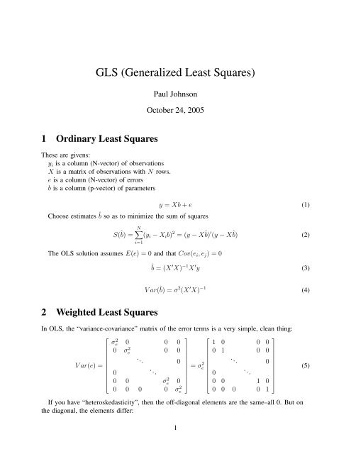
In OLS, the “variance-covariance” matrix of the error terms is a very simple, clean thing:
⎡
σe 2 ⎤ ⎡
⎤
0 0 0 1 0 0 0
0 σe 2 0 0
0 1 0 0
. .. . 0
. ..
= σe
2 .. 0
⎥ ⎢
. ..
⎥
V ar(e) =
⎢
⎣
0
0 0 σe 2 0
0 0 0 0 σe
2
⎥
⎦
0
⎢
⎣
0 0 1 0
0 0 0 0 1
⎥
⎦
(5)
If you have “heteroskedasticity”, then the off-diagonal elements are the same–all 0. But on
the diagonal, the elements differ:
1

⎡
V ar(e) =
⎢
⎣
In weighted least squares, we use estimates of σ 2 e i
σe 2 ⎤
1
0 0 0
0 σe 2 2
0 0
. .. 0
.
0
..
0 0 σe 2 ⎥
N−1
0 ⎦
0 0 0 0 σe 2 N
as weights.
(6)
S(ˆb) =
N∑
i=0
1
̂σ 2 e i
(y i − ŷ i ) 2 =
Consider the WLS problem. If the heteroskedastic case occurs
N∑
w i (y i − ŷ i ) 2 (7)
i=0
N∑
N∑
S(ˆb) = w i (y i − ŷ i ) 2 = ( √ w i y i − √ w i ŷ i ) 2 (8)
i=1
i=1
= w 1 (y 1 − ŷ 1 ) 2 + w 2 (y 2 − ŷ 2 ) 2 + · · · + w N (y N − ŷ N ) 2 (9)
3 Generalized Least Squares (GLS)
Suppose, generally, the Variance/Covariance matrix of residuals is
⎡
σ1 2 Cov(e 1 , e 2 ) Cov(e 1 , e 2 ) · · · Cov(e 1 , e N )
Cov(e 1 , e 2 ) σ2
2 σ3
2
V =
. .
..
⎢
⎣
σN−1 2 Cov(e 1 , e N−1 )
Cov(e 1 , e N ) Cov(e 1 , e N−1 σN
2
⎤
⎥
⎦
(10)
You can factor out a constant σ 2 if you care to (MM&V do, p. 51).
If all the off diagonal elements of V are set to 0, then this degenerates to a problem of heteroskedasticity,
know as Weighted Least Squares (WLS).
If the off diagonal elements of V are not 0, then there can be correlation across cases. In a
time series problem, that amounts to “autocorrelation.” In a cross-sectional problem, it means
that various observations are interrelated.
The “sum of squared errors” approach uses this variance matrix to adjust the data so that the
residuals are homoskedastic or that the cross-unit correlations are taken into account.
Let
W = V −1 (11)
The idea behind WLS/GLS is that there is a way to transform y and X so that the residuals
are homogeneous, some kind of weight is applied.
2

In matrix form, the representation of WLS/GLS is
S(ˆb) = (y − ŷ) ′ W (y − ŷ) (12)
and, if you write that out, the sum of squares in a GLS framework is a rather more complicated
thing. All of those off-diagonal w ij ’s make the number of terms multiply.
⎡
⎤ ⎡
⎤
w 11 w 12 · · · w 1N y 1 − ŷ 1
[ ]
w 12 w 22 w 2N
y 2 − ŷ 2
y1 − ŷ 1 y 2 − ŷ 2 · · · y N − ŷ N ⎢
⎣ .
.. .
⎥ ⎢
⎥
. ⎦ ⎣ . ⎦
w N1 w N2 · · · w NN y N − ŷ N
= [ ]
y 1 − ŷ 1 y 2 − ŷ 2 · · · y N − ŷ N ⎢
⎣
⎡
w 11 (y 1 − ŷ 1 ) +w 12 (y 2 − ŷ 2 ) · · · +w 1N (y N − ŷ N )
w 12 (y 1 − ŷ 1 ) +w 22 (y 2 − ŷ 2 ) +w 2N (y N − ŷ N )
.
.
.. .
w N1 (y 1 − ŷ 1 ) +w N2 (y 2 − ŷ 2 ) · · · +w NN (y N − ŷ N )
⎤
⎥
⎦
⎡
=
⎢
⎣
w 11 (y 1 − ŷ 1 ) 2 ⎤
+w 12 (y 2 − ŷ 2 )(y 1 − ŷ 1 ) · · · +w 1N (y N − ŷ N )(y 1 − ŷ 1 )
w 12 (y 1 − ŷ 1 )(y 2 − ŷ 2 ) +w 22 (y 2 − ŷ 2 ) 2 +w 2N (y N − ŷ N )(y 2 − ŷ 2 )
.
.. .
⎥
.
⎦
w N1 (y 1 − ŷ 1 )(y N − ŷ N ) +w N2 (y 2 − ŷ 2 )(y N − ŷ N ) · · · +w NN (y N − ŷ N ) 2
w 11 (y 1 − ŷ 1 ) 2 + w 12 (y 2 − ŷ 2 )(y 1 − ŷ 1 ) + · · · + w 1N (y N − ŷ N )(y 1 − ŷ 1 )
= +w 12 (y 1 − ŷ 1 )(y 2 − ŷ 2 ) + w 22 (y 2 − ŷ 2 ) 2 + · · · + w 2N (y N − ŷ N )(y 2 − ŷ 2 )
+w N1 (y 1 − ŷ 1 )(y N − ŷ N ) + w N2 (y 2 − ŷ 2 )(y N − ŷ N ) + · · · + w NN (y N − ŷ N ) 2
Supposing a linear model:
N∑ N∑
= w ij (y i − ŷ i )(y j − ŷ j ) (13)
i=1 j=1
ŷ = Xˆb (14)
The normal equations (the name for the first order conditions) are found by setting the derivatives
of the Sum of Squares with respect to the parameters equal to 0.
for each parameter ˆb j :
∂
∂ˆb j
[(y − ŷ) ′ W (y − ŷ)] = 0
If you insert ŷ = Xb in there and do the math (or look it up in a book :) )
(X ′ W X)ˆb − X ′ W y = 0
The WLS/GLS estimator is the solution:
ˆb = (X ′ W X) −1 X ′ W y (15)
3

and, supposing you divide out a constant communal variance term σ 2 and the ’leftovers’
remain in W , the Var/Cov matrix is
V ar(ˆb) = σ 2 (X ′ W X) −1 (16)
The estimate of ˆb is consistent and has lower variance than other linear estimators.
Please note that the formula 16 ends up with such a small, simple formula because of the
simplifying results that are invoked along the way. Observe (don’t forget that V ar(e) = σ 2 V =
σ 2 W −1 , W = W ′ , and V ar(aW ) = aV ar(W )a ′ .) All the rest is easy.
V ar(ˆb) = V ar[(X ′ W X) −1 X ′ W y] (17)
= V ar[(X ′ W X) −1 X ′ W (Xb + e)] = V ar[(X ′ W X) −1 X ′ W e]
= (X ′ W X) −1 X ′ W [V ar(e)]W ′ X(X ′ W X) −1
4 Robust estimates of V ar(ˆb)
= (X ′ W X) −1 X ′ W (σ 2 W −1 )W ′ X(X ′ W X) −1
= σ 2 (X ′ W X) −1 X ′ W X(X ′ W X) −1
= σ 2 (X ′ W X) −1
The Huber-White “sandwich” estimator of V ar(ˆb) is designed to deal with the problem that
the model W may not be entirely correct.
Ordinarily, what people do is to calculate an OLS model, and then use the “sandwich” estimator
to make the estimates of the standard errors more robust. In an OLS context, we use the
observed residuals:
ê = y − Xˆb (18)
This is an “empirical” estimator, in the sense that “rough” estimates of the correlations among
observations are used in place of the hypothesized values. Huber and White developed this estimator,
which is more likely to be accurate when the assumption about W is wrong. 16
When I get tired of gazing at statistics books and really want to know how things get calculated,
I download the source code for R and some of its libraries and go read their code. Assuming
they get it right, which they usually do, its quite easy to figure how things are actually
done.
In the code for the “car” package by John Fox, for example, there’s an R function hccm that
calculates 5 flavors of heteroskedasticity consistent covariance matrices. The oldest, the original,
the Huber-White formula (version hc 0) works on the hypothesis that one can estimate
V ar(e i ) with (ê 2 i ). So, in the OLS model, the V ar(ˆb)starts out like so:
V ar(ˆb) = (X ′ X) −1 X ′ V ar[e]X(X ′ X) −1
4

= (X ′ X) −1 X ′ (σ 2 eI)X(X ′ X) −1
and we replace the middle part with the empirical estimate of the variance matrix.
In the heteroskedasticity case, that matrix looks like this
⎡
ê 2 ⎤
1 0 0 0 0
0 ê 2 2 0 0 0
. 0 0 .. 0 0
= diag[e · e ′ ]
⎢
⎣ 0 0 0 ê 2 N−1 0
⎥
⎦
0 0 0 0 ê 2 N
The heteroskedasticity consistent estimator is thus:
V ar hc0 (b) = (X ′ X) −1 X ′ {diag[e · e ′ ]}X(X ′ X) −1 (19)
It’s called a “sandwich estimator” because somebody thought it was cute to think of the
matching outer elements as pieces of bread. Its also called the “information sandwich estimator”
because those things on the outside look an awful lot like information matrices.
TODO: In Dobson there are some special formulae for correction of standard errors from
panel studies. Write in all those details.
Seems like every time I turn around somebody suggests a new improvement on robust standard
errors, especially for panel studies. I guess when these get published, all the textbooks
and stat packs will have to be redone.
Edward W. Frees and Chunfang Jin. 2003. “Empirical standard errors for longitudinal data
mixed linear models” University of Wisconsin. for information contact jfrees@bus.wisc.edu
5