Projectile Motion Experiment

MASSACHUSETTS INSTITUTE OF TECHNOLOGY
Department of Physics
Physics 8.01T Fall Term 2004
Introduction
Experiment 2: Projectile Motion
The motion of objects under the influence of gravity near the surface of the earth has
been one of the outstanding problems of physics. The solution that once air resistance is
ignored, all objects near the surface of the earth accelerate uniformly towards the earth
marked the beginning of modern physics. A consequence of this physical fact is that the
acceleration of a projectile is independent of the force that launches the projectile, but the
orbit depends on the exit velocity of the projectile.
You will examine one of two types of projectile motion. In the first experiment,
Falling Ball, a ball rolls and/or slides down a tube, leaving the tube with a certain exit
velocity. The ball follows a nearly parabolic orbit (negligible air resistance) until it strikes
the ground. In the second experiment, Projected Ball, the ball is projected vertically
using a spring-loaded assembly and again follows a parabolic trajectory until it hits the
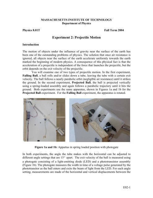
ground. Both experiments use the same apparatus, shown in Figures 1a and 1b for the
Projected Ball experiment. For the Falling Ball experiment, the apparatus is rotated.
Figure 1a and 1b: Appartus in spring loaded position with photogate
In both experiments, the angle the tube makes with the horizontal can be adjusted to
different angle settings that are 15 ° apart. The exit velocity of the ball is measured using
a photogate consisting of a light-emitting diode (LED) and a phototransistor assembly
(Figure 1b). The photogate measures the width in time of a voltage pulse generated by the
phototransitor as the ball enters and exits the beam of light from the LED. For each angle
setting, measurements are made of the horizontal and vertical displacements between the
E02-1

points where the ball exits the tube and where the ball strikes the ground. The direction of
acceleration while in free fall is down with magnitude
g
-2
= 9.8m⋅ s .
In Section 4.4 of the Course Notes, the orbit equation for the parabolic orbit of a
projectile is given by
1 g v
yt =− xt + xt ,
2 y,0
() () ()
2
2 vx,0 vx,0
where the origin of the coordinate system is chosen at the exit point and the direction of
increasing positive y -axis is upwards. The above equation describes both experiments
that utilize the same coordinate system shown in Figures 2a (Falling Ball) and 2b
(Projected Ball). Note that in Figure 2a, the coordinate function yt () ≤ 0and θ0 ≤ 0 .
Figure 2a and 2b: Coordinate system for two types of projectile motion
Since the components of the exit velocity are given by
v = v cosθ
x,0 0 0
v = v sinθ
,
y,0 0 0
the orbit equation can be rewritten as
1 g
yt =− xt + xt .
2
() () tan θ
2 2
0
()
2 v0 cos θ0
If we measure the horizontal displacement, x()
t , the vertical displacement,
initial angle,
velocity,
θ
0
, and we assume the value of
v
=
0 2
yt (), and the
g , we can solve this equation for the initial
2
gxt ()
2cos θ tan ( ) ( )
( θ x t − y t )
0 0
.
E02-2

If we measure the horizontal displacement, x()
t , the vertical displacement, yt (), the
initial angle, θ
0
, and the initial speed v 0
, we can solve this equation for the gravitational
constant g ,
2
v0
g = 2cos tan ( ) − ( )
2
xt ()
2
( θ0( θ0
x t y t ))
Question 1 (answer in the report sheet at the end): In the above expressions for
and g give unusual results if ( tan θ0
xt ( ) − yt ( ) < 0 . Why, on physical and geometric
grounds, can this possibility be excluded?
Idea of the Experiments:
In both experiments (Falling Ball, Projected Ball), you will start out by
assuming that the trajectory of the falling or projected ball follows the trajectory
predicted by constant acceleration in the vertical direction,
)
.
v 0
ay
-2
= − g =−9.8 m ⋅ s .
You will then calculate the exit velocity of the ball from the tube, using the above
equation for the initial velocity.
You will also examine the voltage pulse generated by the photogate as the ball
exits across the light beam. The key step is to calibrate the photogate at the end of the
tube so that you can use information from the voltage pulse to compute the exit velocity.
You can use the reproducible pulse width in time, ∆ T , to calculate an average exit
velocity of the ball,
to compare with the theoretical prediction
vexit
= D ∆ T ,
You will then repeat the experiment, using a different initial angle θ 0
, but this time you
will use your measurements of the horizontal displacement, x()
t , the vertical
displacement, yt (), and the initial angle, θ
0
, and the initial speed v 0
= v ex it
, to calculate
the gravitational constant g .
Experiments:
E02-3

The three groups at each table will do one or other of the two experiments. For either
experiment,
1. Start DataStudio by opening a new DataStudio window and choosing “Create
Experiment.”
2. Connect the Voltage Sensor to Analog Channel A.
3. Add the Voltage Sensor on Data Studio to Channel A by clicking on the Voltage
Sensor Icon in the Experiment Setup window and dragging to “Channel A” on the
image of the 750.
4. Double-click on the Voltage Sensor icon. On the Sensor Properties, set the
Sample rate to 4000 HZ and the Sensitivity to Low.
5. On the Sampling Options choose
• Delayed Start
• Data measurement Voltage is Above 4.000 V
• Keep data prior to start condition 0.010 seconds
6. On Sampling Options-Automatic Stop choose
• Time 0.040 seconds (you may want to adjust this, depending on which
experiment you’re doing, and what the initial angle is).
7. Set up a graph of Voltage vs. Time.
You will record the angle of the tube, the height of the exit point of the tube above
the ground and the horizontal distance between the impact point and the exit point of
the tube. This last measurement requires some care. The ball will land on carbon
paper that will leave a mark on a piece of white paper attached to a clipboard placed
on the carpet. Try not to move the clipboard during the experiment. Use the plumb
bob to determine the point on the carpet directly below the exit point from the tube.
Falling Ball Experiment
1. Line up the black lines on the apparatus with the edge of the table.
2. Clamp the apparatus to the table and record the angle of tube with horizontal.
(This will be some multiple of −15
.)
3. Measure the height of the end of the tube above the floor.
4. Locate the point on the floor directly underneath the end of tube using the plumb
bob. Place tape on the floor underneath the end of tube and mark the end of
plumb bob on the tape.
5. Make a trial run to see where ball hits ground. Put the pin in one of the holes in
the tube and put the ball in the tube. Release the ball by removing the pin. Center
the clipboard (approximately) on this contact point.
6. Place the carbon paper and white paper on the clipboard. Use double sided tape to
secure the clipboard to the floor.
7. Start the run on Data Studio and release the ball. Repeat two more times for
a fixed angle setting.
8. Measure the distance from the plumb bob point to the impact point.
9. Record the data in the report sheet at the end (which you will turn in) and in the
Analysis page, which you will take with you to do the problem set.
E02-4

Projected Ball Experiment
1. Line up the black lines on the apparatus with the edge of the table.
2. Clamp the apparatus to the table and record the angle of tube with horizontal.
(This will be some multiple of 15 .)
3. Measure the height of the end of the tube above the floor.
4. Locate the point on the floor directly underneath the end of tube using the plumb
bob. Place tape on the floor underneath the end of tube and mark the end of
plumb bob on the tape.
5. Make a trial run to see where ball hits ground. Make sure the spring is cocked, put
the ball in the tube and then release the spring. Center the clipboard
(approximately) on this contact point.
6. Place the carbon paper and white paper on the clipboard. Use double sided tape to
secure the clipboard to the floor.
7. Start the run on Data Studio and release the ball by removing the pin
holding the ball in place. Repeat two more times for a fixed angle setting.
8. Measure the distance from the plumb bob point to the impact point for each trial.
9. Record the data in the report sheet at the end (which you will turn in) and in the
Analysis page, which you will take with you to do the problem set.
Question 2 (answer in the report sheet at the end): What role does friction play in your
measurements? How would your results be changed if the tube were completely
frictionless?
Calculation of the Initial Speed Using DataStudio:
“Calibration” of the Photogate
Each of the above trials should have generated a voltage pulse in your DataStudio graph
of Voltage vs. Time. The voltage pulse should have a somewhat trapezoidal shape similar
to that shown in figure 3a.
Figure 3a 3b: Pulse shape for photogate and geometry of ball and beam
E02-5

The rise and fall time is δt . The “flat top” lasts a time interval ∆ t . In order to calibrate
the photogate for use as a velocity meter, you must determine what is the proper time
interval to use for ∆T . Our experience has been that the pulses are rarely as symmetrical
as in the idealization of Figure 3a, and, depending on which apparatus you use, δ t as
shown in Figure 3a may be greatly exaggerated. So, use for ∆ T the FWHM (“Full Width
at Half-Maximum”), the width (in time, in this case) of the pulse between the voltages
corresponding to half of the voltage at the “flat top.”
Use the “Smart Tool” feature of the graph display to measure the width of the pulse. The
“Smart Tool” icon is the fourth from the left at the top of the graph window. The best
way to do this is to find the maximum voltage, center the “Smart Tool” box over a point
on the curve corresponding to half of the maximum and dragging a corner of the box to
the other side of the pulse.
Use your measured value for ∆T for each trial and average the results to calculate the
average velocity of the ball as it leaves the end of the tube.
Record the data in the report sheet at the end (which you will turn in) and in the Analysis
page, which you will take with you to do the problem set.
Question 3 (answer in the report sheet at the end): What error does your method for
measuring the pulse width introduce into your measurement for the average velocity of
the ball? What contribution does the width of the beam make? Can you estimate this
effect? How does this error compare with other errors in the experiment?
Data Analysis:
The analysis will be part of your second problem set.
Calculation of the Gravitational Constant:
Repeat the experiment for a different angle, recording the data in the Analysis page.
This analysis will also be part of your second problem set.
E02-6