Experiment 446.6 VIBRATION-ROTATION SPECTROSCOPY OF ...

Experiment 6, page 1 Version of May 14, 2009
Experiment 446.6
VIBRATION-ROTATION SPECTROSCOPY
OF DIATOMIC MOLECULES
IMPORTANT: The cell should be stored in the dessicator when not in use to prevent
moisture in the atmosphere (Yes, this is Delaware!!!) from injuring the cell windows.
Theory
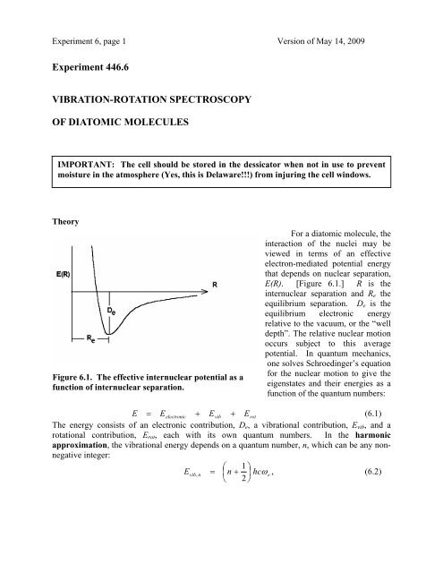
Figure 6.1. The effective internuclear potential as a
function of internuclear separation.
For a diatomic molecule, the
interaction of the nuclei may be
viewed in terms of an effective
electron-mediated potential energy
that depends on nuclear separation,
E(R). [Figure 6.1.] R is the
internuclear separation and R e the
equilibrium separation. D e is the
equilibrium electronic energy
relative to the vacuum, or the “well
depth”. The relative nuclear motion
occurs subject to this average
potential. In quantum mechanics,
one solves Schroedinger’s equation
for the nuclear motion to give the
eigenstates and their energies as a
function of the quantum numbers:
E = Eelectronic + Evib + Erot
(6.1)
The energy consists of an electronic contribution, D e , a vibrational contribution, E vib , and a
rotational contribution, E rot , each with its own quantum numbers. In the harmonic
approximation, the vibrational energy depends on a quantum number, n, which can be any nonnegative
integer:
⎛ 1 ⎞
Evib, n
= ⎜n
+ ⎟ hcω
e
, (6.2)
⎝ 2 ⎠

Experiment 6, page 2 Version of May 14, 2009
for which c is the speed of light in free space, and ω e is the fundamental vibrational frequency
determined by the force constant, k, and the reduced mass, µ. 1
1 k
ω
e
= . (6.3)
2πc
µ
The energy in equation (6.2) is correct only if the molecule is subject to a harmonic
k
potential [i.e. V x
2
= ( − xeq ) ]. One can release this assumption through inclusion of
2
anharmonic terms to give a more complete description of the vibrational energy. The resulting
expression for the vibrational energy is a sum of contributions:
2
⎛ 1 ⎞ ⎛ 1 ⎞ ⎛ 1 ⎞
En
= ⎜n
+ ⎟ω e
− ⎜n
+ ⎟ xeω
e
+ ⎜n
+ ⎟ yeω
e
+ ...... (6.4)
⎝ 2 ⎠ ⎝ 2 ⎠ ⎝ 2 ⎠
The additional terms contain energy parameters x e ω e , y e ω e , .... that account for the anharmonicity
of the potential function. Usually only the first correction term is of significance and the sum is
truncated with only the harmonic and first anharmonic terms. Typical data for several diatomic
molecules are given in Table 6.1.
Table 6.1. Ground-state Spectroscopic Constants of Selected Diatomic Molecules a
Molecule ω e /cm -1 x e ω e /cm -1 B e /cm -1 α e /cm -1
1 H 2 4395.2 117.91 60.81 2.993
12 C 16 O 2170.21 13.461 1.9314 0.01748
1 H 79 Br 2649.67 45.21 8.473 0.226
1 H 19 F 4138.52 90.069 20.939 0.770
2 H 19 F 2998.25 45.71 11.007 0.293
a J. H. Noggle, Physical Chemistry, 3 rd Edition, Addison-Wesley-Longmans, New York, 1996.
3
Vibrational Spectroscopy
When a sample is put in contact with a radiation field, it may take up or emit energy by
having molecules change state. The energy exchange only occurs if the energy spacing in the
molecule is equal to the quantum of energy of the field, ω .
E
final
− Einitial
= ω
(6.5)
For the moment consider only changes in vibrational energy of a diatomic molecule such
as HCl or CO. 2 For most molecules, hcω e

Experiment 6, page 3 Version of May 14, 2009
Since the ground state is so heavily populated under typical conditions, the dominant feature of
vibrational spectroscopy is the transition from n = 0 to n = 1, called the fundamental. To within
the first anharmonic correction, the energy of the photon necessary to excite this transition is:
∆ Evib
= ω
e
− 2xeω
e
. (6.7)
Transitions in which the energy changes by more than 1 quantum are allowed. For example,
the n = 0 → n = 2 transition is known as the first overtone and occurs at an energy:
∆ Eovertone
= 2ω e
− 6xeω
e
(6.8)
to the same level of approximation.
Single-quantum (∆n = ± 1) transitions from states with n > 0 are allowed, but the smaller
populations of these states make such transitions less intense and more difficult to observe at
room temperature. For example, the transition from the state with n = 1 to the state with n = 2
occurs at
∆ Ehot
= ω
e
− 4xeω
e
(6.9)
This is close to the fundamental. Such transitions are called hot bands because their intensities
increase (relative to the fundamental) as one increases the temperature.
Inclusion of Rotational Transitions
In the foregoing discussion, changes in rotational energy were neglected. To analyze
infrared spectra properly, one must consider the effects of rotational-energy changes, as well as
vibrational-energy changes. In the rigid-rotor approximation, the rotational energy of a diatomic
molecule depends on the rotational quantum number, J, as follows.
2
h 1
E rot , Jm
=
2
2 µ R
J ( J + 1) , (6.10)
where the energy, in this equation, is in ergs or joules.
indicates an average over the vibrational wavefunction. As a first approximation, one
1
treats this as
2
R
e
, where R e is the equilibrium bond distance, given by the minimum in the
potential energy curve of Figure 6.1. The equilibrium moment of inertia I (= µR 2 e ) and the
equilibrium rotational constant, B e , are defined in terms of this quantity.
B e
=
h
4πIc
(6.11)
and Erot , Jm
= Be
J ( J + 1)
, (6.12)
where the energy and B e are expressed in cm -1 .
Note that the rotational constant of a molecule depends on the moment of inertia, which
in turn depends on the reduced mass and the equilibrium bond length. The reduced mass
depends on the mass of each isotope. In Table 6.2 are the exact masses of several atoms
(expressed on a molar basis).
Table 6.2. Exact Masses of Several Atoms
Atom Mass (g/mol) Atom Mass (g/mol)
1 H 1.0078250
16 O 15.9949146
2 H (D) 2.0141018
17 O 16.9991312
12 C 12 (exactly)
35 Cl 34.9688527
13 C 13.0033548
37 Cl 36.9659026

Experiment 6, page 4 Version of May 14, 2009
For a real diatomic molecule, the average over the vibrational state means that the
rotation constant is not exactly B e , but instead depends on vibrational state. The rotational
constant including the correction for the vibrational state is given the symbol B n , where the
explicit dependence on the vibrational state is indicated by the subscript. In this way, the
rotational energy of a diatomic molecule in a state with quantum numbers, n, J and m is given
by:
EnJm = Bn
J ( J +1)
(6.13)
Perturbation theory gives the vibration-dependent rotation constant, in a first approximation, as:
⎛ 1 ⎞
Bn = Be
− α
e ⎜n
+ ⎟ . (6.14)
⎝ 2 ⎠
α e is the vibration-rotation constant that describes how the vibrational state affects the rotational
energy. In analyzing spectra, it is treated as a parameter to be determined, just like B e .
In addition to this correction, there is another purely rotational perturbation that changes
the rotational energy of a state - the centrifugal distortion. This is taken into account by an
additional term in the energy that is determined by the centrifugal distortion coefficient, D c .
With all these definitions, the total internal energy of a diatomic molecule in a state with
quantum numbers n, J and m is:
2
En,
Jm ⎛ 1 ⎞ ⎛ 1 ⎞
2 2
= De
+ ⎜n
+ ⎟ω e
− ⎜n
+ ⎟ xeω
e
+ Bn
J ( J + 1) − Dc
J ( J + 1) (6.15)
hc
⎝ 2 ⎠ ⎝ 2 ⎠
Because the energy separations of the rotational states (each having a different value of J)
may not be much greater than k b T, a sample may contain appreciable numbers of molecules in
excited rotational states, even at room temperature. Thus, when rotational energies are
considered, transitions from states with various values of J are seen in a spectrum.
Vibration-Rotation Spectroscopy
Infrared spectroscopy concerns changes of vibrational and rotational state, without
change of electronic state. Hence, the infrared spectrum is a vibration-rotation spectrum. The
usual selection rules are:
• ∆n = ± 1 (Transitions of higher order are known as overtone bands and occur at
higher frequencies; we shall not consider them further here, except in the Discussion
Questions.)
• ∆J = ± 1 (for the heteronuclear diatomic molecules examined here)
• The molecule must have a permanent dipole.
Considering only transitions that involve the ground vibration state, the energy change is:
α
e
∆E
= ωe
− 2xeωe
+ Be
[ J'(
J'
+ 1) − J(
J + 1) ] − [ 3J'(
J'
+ 1) − J(
J + 1) ]
2
(6.16)
2 2 2 2
− Dc[
J'
( J'
+ 1) − J ( J + 1) ]
with the quantum number of the initial rotational state being J and that of the final rotational
state being J’. When J′ = J + 1, there is a net absorption of rotational energy; when J′ = J – 1,
there is a net emission of rotational energy (although overall there is absorption of energy).
Transitions of the former kind form the R branch and those of the latter form the P branch of

Experiment 6, page 5 Version of May 14, 2009
the spectrum. 4 Using equation (6.16), the approximate energies of transition depend on the
quantum number J for the initial state. Neglecting the centrifugal distortion terms, this gives:
2
∆E
= ω (1 − 2x
) + 2( B − α )( J + 1) − α ( J + 1) R branch
e
e
e
e
2
∆E
= ω
e
(1 − 2xe
) − 2( Be
+ α
e
) J − α
e
J
P branch
The infrared spectrum consists of a series of transitions due to the different rotational
states involves. One apparent quality of such a spectrum is the variation in intensity of these
lines. The intensity distribution gives the relative probabilities of occupation of the initial
rotational states (those with quantum number J). From these intensities, one can define a
rotational temperature, T r , for the distribution, assuming it to be Boltzmann in form. The
intensity of a line that arises from the state with quantum number J (compared to that for the line
that comes from a state with J = 0) is given by the following equation that accounts for the
Boltzmann factor and the degeneracy of the rotational level.
I
J
N
J
g
J
= = exp[ −(
EJ
− E0
) / kbTr
] = (2J
+ 1) exp[ −BnhcJ
( J + 1) / kbTr
] (6.18)
I
0
N
0
g
o
A comparison of intensities allows one to estimate T r ; or, knowing T r , one may estimate
B n . In some experiments in which systems are perturbed by laser excitation, one can change the
distribution of molecules in the rotational states (at least for a sufficiently long time to make a
measurement) such that the “rotational temperature” is different from the laboratory temperature.
The use of the intensity distribution can be used to predict the T r . Under the conditions of this
experiment, the rotational degrees of freedom are in equilibrium with the translational degrees of
freedom and the rotational temperature is the same as the laboratory temperature.
e
(6.17)
Quantum Calculations
The theory above assumes that the potential energy function is known or can be
approximated. In actuality, this function is an integral over the electronic wave function of the
molecule. Thus, empirical parameters that describe the function like the force constants are
related to integrals over the electronic state of the molecule. To calculate these, one must have
knowledge of the electronic state of the system. With present-day computers, one may do
numerical estimations of the electronic wave functions rather easily and with quite good
precision. 5 Once known, the functions can be numerically integrated to give estimates of the
values of parameters such as the force constant, k, or the fundamental frequency, ω e , based on
that estimates of the wavefunctions for that particular electronic state.
Many complex operations involved in such calculations have been collected into
“canned” programs such as GAUSSIAN03 6 or SPARTAN, so that the chemist can use the
computer without dealing with problems of computer programming or numerical analysis.
However, there is a great deal of chemical knowledge one must still bring to bear on the process
to obtain reliable results.
4 In spectra of diatomic molecules, the transition for which ∆J = 0 is not allowed. This transition is called the Q
branch of the spectrum. For more complex molecules, this transition may be allowed, and a Q branch may be part
of the spectrum, showing as an intense transition between the R and P branches.
5 Only a few years ago, such calculations were only done by a rather small number of experts on rather large
computers. Today they may be done with the aid of a personal computer at one’s desk.
6 John Pople was awarded the 1998 Nobel Prize in Chemistry principally for the development of GAUSSIAN.

Experiment 6, page 6 Version of May 14, 2009
The principal problem one must cope with in carrying out ab initio quantum calculations
is that any procedure uses some approximation to the molecular electronic wave function(s).
The quality of the approximation determines how good calculated properties are. A commonly
used method is linear combination of atomic orbitals (LCAO), in which one expresses the
molecular electronic wave function (or molecular orbital [MO]) in terms of atomic orbitals of the
constituent atoms. Since the forms of atomic orbitals are not well known except for hydrogen,
even the choice of functional forms of atomic orbitals is an approximation whose quality will
affect the results. The set of functions used is called the basis. A commonly used basis is the
Slater-type orbitals (STO), but other bases are sometimes used, for example Gaussian-type
orbitals. These have esoteric acronyms that denote certain features of the set of orbitals, such as
3-21G or 6-31G or 6-311+G(d,p). In principle, an infinitely large basis set allows one to solve
the electronic state exactly. However, that would take a great amount of time, so that
calculations are always done with a truncated basis; again, the quality of the results depends on
how well the truncated set can be used to approximate the real wave function.
Once chosen, the basis is used to determine the “best” electronic wave function by some
criterion, such as minimization of energy. A common method is the Hartree-Fock self-consistent
field (HF-SCF) method, which emphasizes the average effects of interelectronic interactions,
rather than instantaneous interactions. This iterative method finds parameters of the expansion
of the molecular orbital that minimize the variational energy integral. Conveniently, computer
programs like GAUSSIAN will do all of the work if one describes the desired basis and situation
appropriately, returning useable information on the state in the form of parameters.
CAUTION: HCl and DCl are corrosive gases. ALWAYS handle the materials
extremely carefully.
Procedure
Obtaining the Infrared Spectra
The instrument for measuring the spectra is a Nicolet Magna IR 550 FTIR spectrometer.
If you have not already learned how to use this instrument, your laboratory instructor will help
you with the operating parameters for the instrument. If you have taken instrumental analysis,
this instrument will be familiar to you. This instrument has a liquid-nitrogen-cooled detector.
Before beginning any spectroscopy, obtain liquid nitrogen and fill the reservoir until liquid
nitrogen overflows the fill hole.
An important part of getting reliable data is positioning the sample. The cell holder must
be positioned accurately to allow the full IR intensity to be detected. Make sure the beam passes
through the center of the cell. Take great care in inserting the sample into the sample
compartment. Do not force the sample to go in, as that may break the sample. Remember that
you must wait after closing the sample compartment to allow the system to be purged; wait at
least two minutes after closing the compartment lid.
When obtaining the spectrum of the mixture of HCl and DCl, record all pertinent data so
you can have them when doing the analysis.

Experiment 6, page 7 Version of May 14, 2009
1. You may wish to take a spectrum of the polystyrene standard as the first thing you do to
assure yourself that the spectrometer is working properly. Follow the procedure of
collecting a background and then taking a spectrum of the sample.
2. For the samples of gases, we have made a cradle into which the cell fits. Install the
cradle carefully. If it does not fit properly, do not force it. Have the laboratory
instructor help you.
3. Before taking the spectrum of the gas, take a spectrum of the empty compartment, using
the same parameters as you intend to use in the experimental measurement. This is done
with the command Collect Background. If you have any problems, you should
immediately take a spectrum of the polystyrene standard to confirm proper operation of
the spectrometer.
4. Carefully insert the cell into the cradle. Again, if it does not fit easily into the space, see
the laboratory instructor before proceeding.
5. Take a spectrum of the HCl/DCl sample using the Collect Spectrum command. Unless
otherwise specified, accept the default values supplied by the program. When asked a
question by the program, reply with “Yes”. Unless otherwise specified, all “click”
operations are done with the left mouse button. HCl is an impurity in DCl that can be
identified because of its lower signals in the spectrum. Be sure this is at a resolution high
enough to identify the sharp features of the R and P bands of both materials.
6. Use subtraction of the background to obtain a reasonable high-resolution spectrum if
necessary. This is done automatically by the software for the Nicolet spectrometer.
7. Look at the spectrum to be certain you see both the bands of the HCl and DCl. There
may be other bands from a bit of water vapor in the compartment, and there are some
bands from the epoxy that holds the windows on some cells. The important point to
consider is whether you can detect the spectra of HCl and DCl easily.
8. When you have the spectrum recorded, save the data on a 3.5” floppy disk or on a flash
drive so that you may analyze the data later. Use the Save As command, being sure the
file type is CSV. You should be able to import this file into a program like EXCEL on
your computer for creating a graph and precisely reading the peak positions.
9. Obtain a spectrum of the CO sample in the same manner.
10. Sign the logbook.
Calculational Chemistry
The calculations are done on PCs in the laboratory. There are two operations: (1) setting
up the calculation with GaussView, and (2) running a Gaussian calculation with Gaussian03.
Subsequently one can view the results with GaussView. Start the PC, using the password
provided.
1. Click on the GaussView icon. This should display the main menu of GaussView.

Experiment 6, page 8 Version of May 14, 2009
Atom
Icon
Bond
Length
Inquire
Current
Fragment
“New” file
Window
2. To build the HCl molecule. Click on the atom icon of the main display; this gets you to
the periodic table. Then click on the “Cl” on this display. Close the Select Element
display. You should see an HCl molecule in the Current Fragment display.
3. Click on the “New” file window and this should put a copy of the HCl molecule into your
new file.
4. Click on the bond length icon on the main menu. This will cause the Current Fragment
display to become white. Go to the HCl window. Click first on either the H or Cl atom
and then on the other. A window should open with a slider to set the length of the bond.
Set it at some distance (in Angstrøm units) such as 1.35.
5. Go to the Calculate menu and select Gaussian. This will bring up the Calculate menu in
a window with various tabs. Make sure that the Calculation Type is Energy under the
Job Type tab. In the Title tab, you may type a title such as “HCl, 1.35 A”. Leave
everything else at Default.
6. Submit the job. The program will ask you to save an input file. Use a name like HCl135.
Make certain it is saved as a Gaussian job file on the desktop of the computer. The
calculation should start at this point. This calculation uses the Hartree-Fock
approximation, which gives a reasonably good approximate solution to Schrödinger’s
equation.
7. When the calculation is done (about a minute for this work), the computer opens a
window telling you the job is finished. You may click “Yes” to close the Gaussian
window. From GaussView a box will pop up asking if you want to open the file, click

Experiment 6, page 9 Version of May 14, 2009
“Yes” to open the file. You must indicate that the output file ends with the extension .log
or .out to get output. You can read the file from GaussView using the Results menu. You
may simply click on Summary, which will cause a box with pertinent results to be
shown. You may view the entire file as well.
8. If you are looking at the full file, the output begins with a lot of preliminary stuff. Search
the file to find the line that begins with SCF Done. The quantity called E(RHF) is the
calculated energy of the molecule, in atomic units, a. u. or hartrees.7 This reported energy
is the total energy, that is, the energy required to separate all of the electrons and nuclei to
infinity. Record this number along with the internuclear separation in your notebook.
9. Repeat this calculation for a series of different bond lengths. It is easiest to call back in
the first file you made, click on the two atoms after clicking on the bond length icon and
setting the new length. Save the file with a unique name that will help you to identify
which file corresponds to which bond length upon starting the Gaussian calculation. Use
a set of bond lengths such as 1.35 Å, 1. 45 Å, 1.40 Å, 1.30 Å, 1.25 Å, 1.20 Å, 1.15 Å.
10. With a file having the bond length giving the lowest energy above, set up a new
calculation, choosing Opt+Freq. This will do an optimization and a frequency
calculation. When this calculation is finished be sure to record the optimized bond length
(click on the Inquire button, then on the two atoms) and the dipole moment from the
Summary. This calculation reports the vibrational frequency of HCl in wavenumbers and
the rotational constant. Be sure to record these numbers from the results, as they need to
be reported. The vibrational frequency can be found in the Results menu under
Vibrations. To find the rotational constant you will have to view the whole log file.
Under the Results menu, click View File. This will open the log file and you will need
to scroll down towards the end and look for Thermochemistry.
11. When you finish, delete all of the files from the Desktop that you created, empty the
Recycle Bin and turn off the computer.
Calculations
Data Analysis of the Spectroscopic Results
1. Analysis of HCl Spectra
a. Make a table for 1 H 35 Cl and 1 H 37 Cl of the positions of the lines (in cm -1 ) and the
corresponding values of J. 7 [This can be conveniently done with a computer
program such as Excel.]
b. On one graph, plot the line positions of transitions in the R branch versus J + 1
and the line positions of transitions in the P branch versus J. [Use a dummy
index, m, for J + 1 and J to make these plots.]
c. By multiple-regression analysis of the plots for both species, determine ω e -2x e ω e ,
B e , and α e for each material. (You should do the analysis for both the R and P
branches and assume D c is zero.) 8
2. There are several other ways to analyze these data. Physical chemists like to find ways to
make a linear plot to obtain data. One way to analyze data is via differences between line
positions of adjacent lines in a series. This is particularly useful when the equation is of
7 J is the rotational quantum number of the initial rotational state in each case. Be careful.
8 Be sure to include estimates of uncertainty in your values for these parameters.

Experiment 6, page 10 Version of May 14, 2009
higher order than 1 or 2. Show that the difference between adjacent lines in the R and P
branches are given by the following equations, using equation (6.17):
R branch : ω
J + 1
−ω
J
= 2Be
− 5α
e
− 2α
e
J
. (6.19)
P branch : ω
J
− ω
J + 1
= 2Be
+ 3α
e
+ 2α
e
J
Plot the difference in the lines in the two branches for HCl versus J and extract values of
B e and α e for 1 H 35 Cl and 1 H 37 Cl by this method.
3. Make a table of line positions for each DCl species and analyze these data by either the
method of question 1 or question 2. If you use the second method, you must decide how
to obtain ω e - 2x e ω e .
4. Do an analysis of the spectrum of CO by one of these methods.
5. Summarize all derived results on all gases in a single table. In particular, show the values
of parameters derived for HCl and DCl by both method 1 and method 2.
Theoretical Chemistry
6. From the results of step 8 of the Gaussian03 calculations, make a table of bond length
and energy. In the table indicate whether increasing or decreasing the bond length lowers
the energy at each step of your calculation.
7. Make a plot of calculated energy versus bond length.
8. Compare the optimal bond length determined in the optimization calculation with the
value, Re, from your analysis of the IR experiment, with the determined value in the
single-point calculations and with literature data.
9. Find the dipole moment at the optimal bond length predicted by this calculation.
Compare it with a literature value. [Be sure to quote your literature source.]
10. Compare the calculated values of ω e for HCl to your experimental value and the
literature value. The calculated frequency will be larger than the experimental value.
There is a systematic error in the Hartree-Fock predictions of the frequency, making the
calculated values about 10% too high for all vibrations. A survey of many calculations
produces an empirical correction factor of 0.9085. Apply this correction to your
calculated results and compare with the literature and your experimental values.
Discussion Questions
1. Derive equations (6.7) and (6.8).
2. What are the spectroscopic effects of 35 Cl and 37 Cl? Explain your result by calculating
the first five transitions in the R and P branches of H 35 Cl and H 37 Cl.
3. Calculate the moments of inertia of each of the four possible species in the HCl/DCl
sample from the rotational constants, B e , you determined.
4. From each moment of inertia, calculate R e for each of the four isotopomers. Within
experimental error, are these bond distances different from each other? Explain your
answer.
5. The expected position of the Q branch of HCl is different from that of DCl. What are
your experimental values for these? Assuming that the anharmonic term is zero,
calculate the ratio of the reduced masses of 1 H 35 Cl and 2 H 35 Cl from you data for the
expected positions of the Q branch. How does this agree with literature data for this
quantity?

Experiment 6, page 11 Version of May 14, 2009
6. Convert your calculated value of the energy (from the GAUSSIAN calculation) to
kcal/mol and compare it with the dissociation energy of HCl, D(HCl), from an
appropriate reference.
7. Explain why the IR cell is constructed the way it is. In particular, why is it not made
completely out of glass?
8. Uncertainty in FTIR depends on the noise at the detector. 9 In many infrared
spectrometers, the signal is a ratio of the detected response to a reference response.
Explain, with equations if necessary, why it is necessary to consider the noise in the
reference channel as well as the noise in the detector channel when calculating signal-tonoise
ratios in FTIR experiments. In what kinds of experiments will this be of concern?
9 H. L. Mark and P. R. Griffiths, “Analysis of Noise in Fourier Transform Infrared Spectra”, Applied Spectroscopy,
56, 633-639 (2002).