Introduction to Probability and Statistics Using R - Youngstown State ...

Introduction to Probability
and Statistics Using R
G. Jay Kerns
First Edition

ii
IP S UR: Introduction to Probability and Statistics Using R
Copyright © 2011 G. Jay Kerns
ISBN: 978-0-557-24979-4
Permission is granted to copy, distribute and/or modify this document under the terms
of the GNU Free Documentation License, Version 1.3 or any later version published by
the Free Software Foundation; with no Invariant Sections, no Front-Cover Texts, and no
Back-Cover Texts. A copy of the license is included in the section entitled “GNU Free
Documentation License”.
Date: August 12, 2011

Contents
Preface
List of Figures
List of Tables
vii
xiii
xv
1 An Introduction to Probability and Statistics 1
1.1 Probability . . . . . . . . . . . . . . . . . . . . . . . . . . . . . . . . . . 1
1.2 Statistics . . . . . . . . . . . . . . . . . . . . . . . . . . . . . . . . . . . . 1
Chapter Exercises . . . . . . . . . . . . . . . . . . . . . . . . . . . . . . . . . . 2
2 An Introduction to R 3
2.1 Downloading and Installing R . . . . . . . . . . . . . . . . . . . . . . . . 3
2.2 Communicating with R . . . . . . . . . . . . . . . . . . . . . . . . . . . . 4
2.3 Basic R Operations and Concepts . . . . . . . . . . . . . . . . . . . . . . 6
2.4 Getting Help . . . . . . . . . . . . . . . . . . . . . . . . . . . . . . . . . 12
2.5 External Resources . . . . . . . . . . . . . . . . . . . . . . . . . . . . . . 14
2.6 Other Tips . . . . . . . . . . . . . . . . . . . . . . . . . . . . . . . . . . . 15
Chapter Exercises . . . . . . . . . . . . . . . . . . . . . . . . . . . . . . . . . . 16
3 Data Description 17
3.1 Types of Data . . . . . . . . . . . . . . . . . . . . . . . . . . . . . . . . . 17
3.2 Features of Data Distributions . . . . . . . . . . . . . . . . . . . . . . . . 32
3.3 Descriptive Statistics . . . . . . . . . . . . . . . . . . . . . . . . . . . . . 34
3.4 Exploratory Data Analysis . . . . . . . . . . . . . . . . . . . . . . . . . . 39
3.5 Multivariate Data and Data Frames . . . . . . . . . . . . . . . . . . . . . 44
3.6 Comparing Populations . . . . . . . . . . . . . . . . . . . . . . . . . . . . 46
Chapter Exercises . . . . . . . . . . . . . . . . . . . . . . . . . . . . . . . . . . 53
4 Probability 65
4.1 Sample Spaces . . . . . . . . . . . . . . . . . . . . . . . . . . . . . . . . . 65
4.2 Events . . . . . . . . . . . . . . . . . . . . . . . . . . . . . . . . . . . . . 70
4.3 Model Assignment . . . . . . . . . . . . . . . . . . . . . . . . . . . . . . 76
4.4 Properties of Probability . . . . . . . . . . . . . . . . . . . . . . . . . . . 81
4.5 Counting Methods . . . . . . . . . . . . . . . . . . . . . . . . . . . . . . 85
4.6 Conditional Probability . . . . . . . . . . . . . . . . . . . . . . . . . . . . 91
4.7 Independent Events . . . . . . . . . . . . . . . . . . . . . . . . . . . . . . 97
4.8 Bayes’ Rule . . . . . . . . . . . . . . . . . . . . . . . . . . . . . . . . . . 100
4.9 Random Variables . . . . . . . . . . . . . . . . . . . . . . . . . . . . . . . 103
Chapter Exercises . . . . . . . . . . . . . . . . . . . . . . . . . . . . . . . . . . 107
iii

iv
CONTENTS
5 Discrete Distributions 109
5.1 Discrete Random Variables . . . . . . . . . . . . . . . . . . . . . . . . . . 109
5.2 The Discrete Uniform Distribution . . . . . . . . . . . . . . . . . . . . . 112
5.3 The Binomial Distribution . . . . . . . . . . . . . . . . . . . . . . . . . . 114
5.4 Expectation and Moment Generating Functions . . . . . . . . . . . . . . 119
5.5 The Empirical Distribution . . . . . . . . . . . . . . . . . . . . . . . . . . 123
5.6 Other Discrete Distributions . . . . . . . . . . . . . . . . . . . . . . . . . 125
5.7 Functions of Discrete Random Variables . . . . . . . . . . . . . . . . . . 133
Chapter Exercises . . . . . . . . . . . . . . . . . . . . . . . . . . . . . . . . . . 135
6 Continuous Distributions 139
6.1 Continuous Random Variables . . . . . . . . . . . . . . . . . . . . . . . . 139
6.2 The Continuous Uniform Distribution . . . . . . . . . . . . . . . . . . . . 144
6.3 The Normal Distribution . . . . . . . . . . . . . . . . . . . . . . . . . . . 145
6.4 Functions of Continuous Random Variables . . . . . . . . . . . . . . . . . 149
6.5 Other Continuous Distributions . . . . . . . . . . . . . . . . . . . . . . . 153
Chapter Exercises . . . . . . . . . . . . . . . . . . . . . . . . . . . . . . . . . . 158
7 Multivariate Distributions 161
7.1 Joint and Marginal Probability Distributions . . . . . . . . . . . . . . . . 161
7.2 Joint and Marginal Expectation . . . . . . . . . . . . . . . . . . . . . . . 167
7.3 Conditional Distributions . . . . . . . . . . . . . . . . . . . . . . . . . . . 170
7.4 Independent Random Variables . . . . . . . . . . . . . . . . . . . . . . . 171
7.5 Exchangeable Random Variables . . . . . . . . . . . . . . . . . . . . . . . 174
7.6 The Bivariate Normal Distribution . . . . . . . . . . . . . . . . . . . . . 175
7.7 Bivariate Transformations of Random Variables . . . . . . . . . . . . . . 176
7.8 Remarks for the Multivariate Case . . . . . . . . . . . . . . . . . . . . . 179
7.9 The Multinomial Distribution . . . . . . . . . . . . . . . . . . . . . . . . 182
Chapter Exercises . . . . . . . . . . . . . . . . . . . . . . . . . . . . . . . . . . 184
8 Sampling Distributions 185
8.1 Simple Random Samples . . . . . . . . . . . . . . . . . . . . . . . . . . . 186
8.2 Sampling from a Normal Distribution . . . . . . . . . . . . . . . . . . . . 187
8.3 The Central Limit Theorem . . . . . . . . . . . . . . . . . . . . . . . . . 189
8.4 Sampling Distributions of Two-Sample Statistics . . . . . . . . . . . . . . 191
8.5 Simulated Sampling Distributions . . . . . . . . . . . . . . . . . . . . . . 193
Chapter Exercises . . . . . . . . . . . . . . . . . . . . . . . . . . . . . . . . . . 196
9 Estimation 199
9.1 Point Estimation . . . . . . . . . . . . . . . . . . . . . . . . . . . . . . . 199
9.2 Confidence Intervals for Means . . . . . . . . . . . . . . . . . . . . . . . . 207
9.3 Confidence Intervals for Differences of Means . . . . . . . . . . . . . . . . 214
9.4 Confidence Intervals for Proportions . . . . . . . . . . . . . . . . . . . . . 216
9.5 Confidence Intervals for Variances . . . . . . . . . . . . . . . . . . . . . . 218
9.6 Fitting Distributions . . . . . . . . . . . . . . . . . . . . . . . . . . . . . 218
9.7 Sample Size and Margin of Error . . . . . . . . . . . . . . . . . . . . . . 218
9.8 Other Topics . . . . . . . . . . . . . . . . . . . . . . . . . . . . . . . . . 220
Chapter Exercises . . . . . . . . . . . . . . . . . . . . . . . . . . . . . . . . . . 221

CONTENTS
v
10 Hypothesis Testing 223
10.1 Introduction . . . . . . . . . . . . . . . . . . . . . . . . . . . . . . . . . . 223
10.2 Tests for Proportions . . . . . . . . . . . . . . . . . . . . . . . . . . . . . 224
10.3 One Sample Tests for Means and Variances . . . . . . . . . . . . . . . . . 229
10.4 Two-Sample Tests for Means and Variances . . . . . . . . . . . . . . . . 233
10.5 Other Hypothesis Tests . . . . . . . . . . . . . . . . . . . . . . . . . . . . 235
10.6 Analysis of Variance . . . . . . . . . . . . . . . . . . . . . . . . . . . . . 235
10.7 Sample Size and Power . . . . . . . . . . . . . . . . . . . . . . . . . . . . 237
Chapter Exercises . . . . . . . . . . . . . . . . . . . . . . . . . . . . . . . . . . 239
11 Simple Linear Regression 241
11.1 Basic Philosophy . . . . . . . . . . . . . . . . . . . . . . . . . . . . . . . 241
11.2 Estimation . . . . . . . . . . . . . . . . . . . . . . . . . . . . . . . . . . . 245
11.3 Model Utility and Inference . . . . . . . . . . . . . . . . . . . . . . . . . 254
11.4 Residual Analysis . . . . . . . . . . . . . . . . . . . . . . . . . . . . . . . 259
11.5 Other Diagnostic Tools . . . . . . . . . . . . . . . . . . . . . . . . . . . . 266
Chapter Exercises . . . . . . . . . . . . . . . . . . . . . . . . . . . . . . . . . . 274
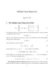
12 Multiple Linear Regression 275
12.1 The Multiple Linear Regression Model . . . . . . . . . . . . . . . . . . . 275
12.2 Estimation and Prediction . . . . . . . . . . . . . . . . . . . . . . . . . . 278
12.3 Model Utility and Inference . . . . . . . . . . . . . . . . . . . . . . . . . 285
12.4 Polynomial Regression . . . . . . . . . . . . . . . . . . . . . . . . . . . . 288
12.5 Interaction . . . . . . . . . . . . . . . . . . . . . . . . . . . . . . . . . . . 292
12.6 Qualitative Explanatory Variables . . . . . . . . . . . . . . . . . . . . . . 294
12.7 Partial F Statistic . . . . . . . . . . . . . . . . . . . . . . . . . . . . . . 297
12.8 Residual Analysis and Diagnostic Tools . . . . . . . . . . . . . . . . . . . 300
12.9 Additional Topics . . . . . . . . . . . . . . . . . . . . . . . . . . . . . . . 301
Chapter Exercises . . . . . . . . . . . . . . . . . . . . . . . . . . . . . . . . . . 305
13 Resampling Methods 307
13.1 Introduction . . . . . . . . . . . . . . . . . . . . . . . . . . . . . . . . . . 307
13.2 Bootstrap Standard Errors . . . . . . . . . . . . . . . . . . . . . . . . . . 309
13.3 Bootstrap Confidence Intervals . . . . . . . . . . . . . . . . . . . . . . . 314
13.4 Resampling in Hypothesis Tests . . . . . . . . . . . . . . . . . . . . . . . 316
Chapter Exercises . . . . . . . . . . . . . . . . . . . . . . . . . . . . . . . . . . 319
14 Categorical Data Analysis 321
15 Nonparametric Statistics 323
16 Time Series 325
A R Session Information 327
B GNU Free Documentation License 329
C History 337
D Data 339

vi
CONTENTS
D.1 Data Structures . . . . . . . . . . . . . . . . . . . . . . . . . . . . . . . . 339
D.2 Importing Data . . . . . . . . . . . . . . . . . . . . . . . . . . . . . . . . 344
D.3 Creating New Data Sets . . . . . . . . . . . . . . . . . . . . . . . . . . . 345
D.4 Editing Data . . . . . . . . . . . . . . . . . . . . . . . . . . . . . . . . . 345
D.5 Exporting Data . . . . . . . . . . . . . . . . . . . . . . . . . . . . . . . . 346
D.6 Reshaping Data . . . . . . . . . . . . . . . . . . . . . . . . . . . . . . . . 347
E Mathematical Machinery 349
E.1 Set Algebra . . . . . . . . . . . . . . . . . . . . . . . . . . . . . . . . . . 349
E.2 Differential and Integral Calculus . . . . . . . . . . . . . . . . . . . . . . 350
E.3 Sequences and Series . . . . . . . . . . . . . . . . . . . . . . . . . . . . . 353
E.4 The Gamma Function . . . . . . . . . . . . . . . . . . . . . . . . . . . . 355
E.5 Linear Algebra . . . . . . . . . . . . . . . . . . . . . . . . . . . . . . . . 356
E.6 Multivariable Calculus . . . . . . . . . . . . . . . . . . . . . . . . . . . . 357
F Writing Reports with R 361
F.1 What to Write . . . . . . . . . . . . . . . . . . . . . . . . . . . . . . . . 361
F.2 How to Write It with R . . . . . . . . . . . . . . . . . . . . . . . . . . . . 362
F.3 Formatting Tables . . . . . . . . . . . . . . . . . . . . . . . . . . . . . . 365
F.4 Other Formats . . . . . . . . . . . . . . . . . . . . . . . . . . . . . . . . 365
G Instructions for Instructors 367
G.1 Generating This Document . . . . . . . . . . . . . . . . . . . . . . . . . . 368
G.2 How to Use This Document . . . . . . . . . . . . . . . . . . . . . . . . . 369
G.3 Ancillary Materials . . . . . . . . . . . . . . . . . . . . . . . . . . . . . . 369
G.4 Modifying This Document . . . . . . . . . . . . . . . . . . . . . . . . . . 370
H RcmdrTestDrive Story 371
Bibliography 377

Preface
This book was expanded from lecture materials I use in a one semester upper-division
undergraduate course entitled Probability and Statistics at Youngstown State University.
Those lecture materials, in turn, were based on notes that I transcribed as a graduate student
at Bowling Green State University. The course for which the materials were written
is 50-50 Probability and Statistics, and the attendees include mathematics, engineering,
and computer science majors (among others). The catalog prerequisites for the course
are a full year of calculus.
The book can be subdivided into three basic parts. The first part includes the introductions
and elementary descriptive statistics; I want the students to be knee-deep in
data right out of the gate. The second part is the study of probability, which begins at
the basics of sets and the equally likely model, journeys past discrete/continuous random
variables, and continues through to multivariate distributions. The chapter on sampling
distributions paves the way to the third part, which is inferential statistics. This last part
includes point and interval estimation, hypothesis testing, and finishes with introductions
to selected topics in applied statistics.
I usually only have time in one semester to cover a small subset of this book. I cover the
material in Chapter 2 in a class period that is supplemented by a take-home assignment
for the students. I spend a lot of time on Data Description, Probability, Discrete, and
Continuous Distributions. I mention selected facts from Multivariate Distributions in
passing, and discuss the meaty parts of Sampling Distributions before moving right along
to Estimation (which is another chapter I dwell on considerably). Hypothesis Testing
goes faster after all of the previous work, and by that time the end of the semester is in
sight. I normally choose one or two final chapters (sometimes three) from the remaining
to survey, and regret at the end that I did not have the chance to cover more.
In an attempt to be correct I have included material in this book which I would
normally not mention during the course of a standard lecture. For instance, I normally do
not highlight the intricacies of measure theory or integrability conditions when speaking
to the class. Moreover, I often stray from the matrix approach to multiple linear regression
because many of my students have not yet been formally trained in linear algebra. That
being said, it is important to me for the students to hold something in their hands which
acknowledges the world of mathematics and statistics beyond the classroom, and which
may be useful to them for many semesters to come. It also mirrors my own experience
as a student.
The vision for this document is a more or less self contained, essentially complete,
correct, introductory textbook. There should be plenty of exercises for the student, with
full solutions for some, and no solutions for others (so that the instructor may assign them
for grading). By Sweave’s dynamic nature it is possible to write randomly generated
exercises and I had planned to implement this idea already throughout the book. Alas,
there are only 24 hours in a day. Look for more in future editions.
vii

viii
CONTENTS
Seasoned readers will be able to detect my origins: Probability and Statistical Inference
by Hogg and Tanis [44], Statistical Inference by Casella and Berger [13], and Theory
of Point Estimation/Testing Statistical Hypotheses by Lehmann [59, 58]. I highly recommend
each of those books to every reader of this one. Some R books with “introductory”
in the title that I recommend are Introductory Statistics with R by Dalgaard [19] and
Using R for Introductory Statistics by Verzani [87]. Surely there are many, many other
good introductory books about R, but frankly, I have tried to steer clear of them for the
past year or so to avoid any undue influence on my own writing.
I would like to make special mention of two other books: Introduction to Statistical
Thought by Michael Lavine [56] and Introduction to Probability by Grinstead and Snell
[37]. Both of these books are free and are what ultimately convinced me to release IP S UR
under a free license, too.
Please bear in mind that the title of this book is “Introduction to Probability and
Statistics Using R”, and not “Introduction to R Using Probability and Statistics”, nor
even “Introduction to Probability and Statistics and R Using Words”. The people at the
party are Probability and Statistics; the handshake is R. There are several important
topics about R which some individuals will feel are underdeveloped, glossed over, or
wantonly omitted. Some will feel the same way about the probabilistic and/or statistical
content. Still others will just want to learn R and skip all of the mathematics.
Despite any misgivings: here it is, warts and all. I humbly invite said individuals to
take this book, with the GNU Free Documentation License (GNU-FDL) in hand, and
make it better. In that spirit there are at least a few ways in my view in which this book
could be improved.
Better data. The data analyzed in this book are almost entirely from the datasets
package in base R, and here is why:
1. I made a conscious effort to minimize dependence on contributed packages,
2. The data are instantly available, already in the correct format, so we need not
take time to manage them, and
3. The data are real.
I made no attempt to choose data sets that would be interesting to the students;
rather, data were chosen for their potential to convey a statistical point. Many
of the data sets are decades old or more (for instance, the data used to introduce
simple linear regression are the speeds and stopping distances of cars in the 1920’s).
In a perfect world with infinite time I would research and contribute recent, real
data in a context crafted to engage the students in every example. One day I hope
to stumble over said time. In the meantime, I will add new data sets incrementally
as time permits.
More proofs. I would like to include more proofs for the sake of completeness (I understand
that some people would not consider more proofs to be improvement). Many
proofs have been skipped entirely, and I am not aware of any rhyme or reason to
the current omissions. I will add more when I get a chance.
More and better graphics: I have not used the ggplot2 package [90] because I do not
know how to use it yet. It is on my to-do list.

CONTENTS
ix
More and better exercises: There are only a few exercises in the first edition simply
because I have not had time to write more. I have toyed with the exams package
[38] and I believe that it is a right way to move forward. As I learn more about
what the package can do I would like to incorporate it into later editions of this
book.
About This Document
IP S UR contains many interrelated parts: the Document, the Program, the Package,
and the Ancillaries. In short, the Document is what you are reading right now. The
Program provides an efficient means to modify the Document. The Package is an R
package that houses the Program and the Document. Finally, the Ancillaries are extra
materials that reside in the Package and were produced by the Program to supplement
use of the Document. We briefly describe each of them in turn.
The Document
The Document is that which you are reading right now – IP S UR’s raison d’être. There
are transparent copies (nonproprietary text files) and opaque copies (everything else).
See the GNU-FDL in Appendix B for more precise language and details.
IPSUR.tex is a transparent copy of the Document to be typeset with a L A TEX distribution
such as MikTEX or TEX Live. Any reader is free to modify the Document and release
the modified version in accordance with the provisions of the GNU-FDL. Note that
this file cannot be used to generate a randomized copy of the Document. Indeed, in
its released form it is only capable of typesetting the exact version of IP S UR which
you are currently reading. Furthermore, the .tex file is unable to generate any of
the ancillary materials.
IPSUR-xxx.eps, IPSUR-xxx.pdf are the image files for every graph in the Document.
These are needed when typesetting with L A TEX.
IPSUR.pdf is an opaque copy of the Document. This is the file that instructors would
likely want to distribute to students.
IPSUR.dvi is another opaque copy of the Document in a different file format.
The Program
The Program includes IPSUR.lyx and its nephew IPSUR.Rnw; the purpose of each is to
give individuals a way to quickly customize the Document for their particular purpose(s).
IPSUR.lyx is the source LYX file for the Program, released under the GNU General Public
License (GNU GPL) Version 3. This file is opened, modified, and compiled with
LYX, a sophisticated open-source document processor, and may be used (together
with Sweave) to generate a randomized, modified copy of the Document with brand
new data sets for some of the exercises and the solution manuals (in the Second
Edition). Additionally, LYX can easily activate/deactivate entire blocks of the document,
e.g. the proofs of the theorems, the student solutions to the exercises, or

x
CONTENTS
the instructor answers to the problems, so that the new author may choose which
sections (s)he would like to include in the final Document (again, Second Edition).
The IPSUR.lyx file is all that a person needs (in addition to a properly configured
system – see Appendix G) to generate/compile/export to all of the other formats
described above and below, which includes the ancillary materials IPSUR.Rdata and
IPSUR.R.
IPSUR.Rnw is another form of the source code for the Program, also released under the
GNU GPL Version 3. It was produced by exporting IPSUR.lyx into R/Sweave format
(.Rnw). This file may be processed with Sweave to generate a randomized copy
of IPSUR.tex – a transparent copy of the Document – together with the ancillary
materials IPSUR.Rdata and IPSUR.R. Please note, however, that IPSUR.Rnw is just
a simple text file which does not support many of the extra features that LYX offers
such as WYSIWYM editing, instantly (de)activating branches of the manuscript,
and more.
The Package
There is a contributed package on CRAN, called IPSUR. The package affords many advantages,
one being that it houses the Document in an easy-to-access medium. Indeed, a
student can have the Document at his/her fingertips with only three commands:
> install.packages("IPSUR")
> library(IPSUR)
> read(IPSUR)
Another advantage goes hand in hand with the Program’s license; since IP S UR is free,
the source code must be freely available to anyone that wants it. A package hosted on
CRAN allows the author to obey the license by default.
A much more important advantage is that the excellent facilities at R-Forge are building
and checking the package daily against patched and development versions of the
absolute latest pre-release of R. If any problems surface then I will know about it within
24 hours.
And finally, suppose there is some sort of problem. The package structure makes it
incredibly easy for me to distribute bug-fixes and corrected typographical errors. As an
author I can make my corrections, upload them to the repository at R-Forge, and they
will be reflected worldwide within hours. We aren’t in Kansas anymore, Toto.
Ancillary Materials
These are extra materials that accompany IP S UR. They reside in the /etc subdirectory
of the package source.
IPSUR.RData is a saved image of the R workspace at the completion of the Sweave processing
of IP S UR. It can be loaded into memory with File ⊲ Load Workspace or with
the command load("/path/to/IPSUR.Rdata"). Either method will make every
single object in the file immediately available and in memory. In particular, the
data BLANK from Exercise BLANK in Chapter BLANK on page BLANK will be
loaded. Type BLANK at the command line (after loading IPSUR.RData) to see for
yourself.

CONTENTS
xi
IPSUR.R is the exported R code from IPSUR.Rnw. With this script, literally every R
command from the entirety of IP S UR can be resubmitted at the command line.
Notation
We use the notation x or stem.leaf notation to denote objects, functions, etc.. The
sequence “Statistics ⊲ Summaries ⊲ Active Dataset” means to click the Statistics menu item,
next click the Summaries submenu item, and finally click Active Dataset.
Acknowledgements
This book would not have been possible without the firm mathematical and statistical
foundation provided by the professors at Bowling Green State University, including
Drs. Gábor Székely, Craig Zirbel, Arjun K. Gupta, Hanfeng Chen, Truc Nguyen, and
James Albert. I would also like to thank Drs. Neal Carothers and Kit Chan.
I would also like to thank my colleagues at Youngstown State University for their
support. In particular, I would like to thank Dr. G. Andy Chang for showing me what it
means to be a statistician.
I would like to thank Richard Heiberger for his insightful comments and improvements
to several points and displays in the manuscript.
Finally, and most importantly, I would like to thank my wife for her patience and
understanding while I worked hours, days, months, and years on a free book. In retrospect,
I can’t believe I ever got away with it.

xii
CONTENTS

List of Figures
3.1.1 Strip charts of the precip, rivers, and discoveries data . . . . . . 20
3.1.2 (Relative) frequency histograms of the precip data . . . . . . . . . . 21
3.1.3 More histograms of the precip data . . . . . . . . . . . . . . . . . . . 22
3.1.4 Index plots of the LakeHuron data . . . . . . . . . . . . . . . . . . . . 25
3.1.5 Bar graphs of the state.region data . . . . . . . . . . . . . . . . . . 28
3.1.6 Pareto chart of the state.division data . . . . . . . . . . . . . . . . 29
3.1.7 Dot chart of the state.region data . . . . . . . . . . . . . . . . . . . 30
3.6.1 Boxplots of weight by feed type in the chickwts data . . . . . . . . 50
3.6.2 Histograms of age by education level from the infert data . . . . . 50
3.6.3 An xyplot of Petal.Length versus Petal.Width by Species in the
iris data . . . . . . . . . . . . . . . . . . . . . . . . . . . . . . . . . 51
3.6.4 A coplot of conc versus uptake by Type and Treatment in the CO2 data 52
4.0.1 Two types of experiments . . . . . . . . . . . . . . . . . . . . . . . . . 66
4.5.1 The birthday problem . . . . . . . . . . . . . . . . . . . . . . . . . . . 90
5.3.1 Graph of the binom(size = 3, prob = 1/2) CDF . . . . . . . . . . . . 117
5.3.2 The binom(size = 3, prob = 0.5) distribution from the distr package 118
5.5.1 The empirical CDF . . . . . . . . . . . . . . . . . . . . . . . . . . . . 124
6.5.1 Chi square distribution for various degrees of freedom . . . . . . . . . 155
6.5.2 Plot of the gamma(shape = 13, rate = 1) MGF . . . . . . . . . . . . 158
7.6.1 Graph of a bivariate normal PDF . . . . . . . . . . . . . . . . . . . . 177
7.9.1 Plot of a multinomial PMF . . . . . . . . . . . . . . . . . . . . . . . . 184
8.2.1 Student’s t distribution for various degrees of freedom . . . . . . . . . 189
8.5.1 Plot of simulated IQRs . . . . . . . . . . . . . . . . . . . . . . . . . . 194
8.5.2 Plot of simulated MADs . . . . . . . . . . . . . . . . . . . . . . . . . 195
9.1.1 Capture-recapture experiment . . . . . . . . . . . . . . . . . . . . . . 201
9.1.2 Assorted likelihood functions for fishing, part two . . . . . . . . . . . 202
9.1.3 Species maximum likelihood . . . . . . . . . . . . . . . . . . . . . . . 203
9.2.1 Simulated confidence intervals . . . . . . . . . . . . . . . . . . . . . . 209
9.2.2 Confidence interval plot for the PlantGrowth data . . . . . . . . . . . 212
10.2.1 Hypothesis test plot based on normal.and.t.dist from the HH package 230
10.3.1 Hypothesis test plot based on normal.and.t.dist from the HH package 232
10.6.1 Between group versus within group variation . . . . . . . . . . . . . . 237
10.6.2 Between group versus within group variation . . . . . . . . . . . . . . 238
10.6.3 Some F plots from the HH package . . . . . . . . . . . . . . . . . . . . 239
10.7.1 Plot of significance level and power . . . . . . . . . . . . . . . . . . . 240
xiii

xiv
LIST OF FIGURES
11.1.1 Philosophical foundations of SLR . . . . . . . . . . . . . . . . . . . . 243
11.1.2 Scatterplot of dist versus speed for the cars data . . . . . . . . . . . 244
11.2.1 Scatterplot with added regression line for the cars data . . . . . . . . 247
11.2.2 Scatterplot with confidence/prediction bands for the cars data . . . . 255
11.4.1 Normal q-q plot of the residuals for the cars data . . . . . . . . . . . 260
11.4.2 Plot of standardized residuals against the fitted values for the cars data 262
11.4.3 Plot of the residuals versus the fitted values for the cars data . . . . . 264
11.5.1 Cook’s distances for the cars data . . . . . . . . . . . . . . . . . . . . 271
11.5.2 Diagnostic plots for the cars data . . . . . . . . . . . . . . . . . . . . 273
12.1.1 Scatterplot matrix of trees data . . . . . . . . . . . . . . . . . . . . . 277
12.1.2 3D scatterplot with regression plane for the trees data . . . . . . . . 278
12.4.1 Scatterplot of Volume versus Girth for the trees data . . . . . . . . . 289
12.4.2 A quadratic model for the trees data . . . . . . . . . . . . . . . . . . 291
12.6.1 A dummy variable model for the trees data . . . . . . . . . . . . . . 297
13.2.1 Bootstrapping the standard error of the mean, simulated data . . . . 310
13.2.2 Bootstrapping the standard error of the median for the rivers data . 312

List of Tables
4.1 Sampling k from n objects with urnsamples . . . . . . . . . . . . . . . . 87
4.2 Rolling two dice . . . . . . . . . . . . . . . . . . . . . . . . . . . . . . . . 92
5.1 Correspondence between stats and distr . . . . . . . . . . . . . . . . . 118
7.1 Maximum U and sum V of a pair of dice rolls (X, Y) . . . . . . . . . . . . 164
7.2 Joint values of U = max(X, Y) and V = X + Y . . . . . . . . . . . . . . . . 164
7.3 The joint PMF of (U, V) . . . . . . . . . . . . . . . . . . . . . . . . . . . 164
E.1 Set operations . . . . . . . . . . . . . . . . . . . . . . . . . . . . . . . . . 349
E.2 Differentiation rules . . . . . . . . . . . . . . . . . . . . . . . . . . . . . . 351
E.3 Some derivatives . . . . . . . . . . . . . . . . . . . . . . . . . . . . . . . 351
E.4 Some integrals (constants of integration omitted) . . . . . . . . . . . . . 352
xv

xvi
LIST OF TABLES

Chapter 1
An Introduction to Probability and
Statistics
This chapter has proved to be the hardest to write, by far. The trouble is that there is
so much to say – and so many people have already said it so much better than I could.
When I get something I like I will release it here.
In the meantime, there is a lot of information already available to a person with an
Internet connection. I recommend to start at Wikipedia, which is not a flawless resource
but it has the main ideas with links to reputable sources.
In my lectures I usually tell stories about Fisher, Galton, Gauss, Laplace, Quetelet,
and the Chevalier de Mere.
1.1 Probability
The common folklore is that probability has been around for millennia but did not gain
the attention of mathematicians until approximately 1654 when the Chevalier de Mere
had a question regarding the fair division of a game’s payoff to the two players, if the
game had to end prematurely.
1.2 Statistics
Statistics concerns data; their collection, analysis, and interpretation. In this book we
distinguish between two types of statistics: descriptive and inferential.
Descriptive statistics concerns the summarization of data. We have a data set and
we would like to describe the data set in multiple ways. Usually this entails calculating
numbers from the data, called descriptive measures, such as percentages, sums, averages,
and so forth.
Inferential statistics does more. There is an inference associated with the data set, a
conclusion drawn about the population from which the data originated.
I would like to mention that there are two schools of thought of statistics: frequentist
and bayesian. The difference between the schools is related to how the two groups interpret
the underlying probability (see Section 4.3). The frequentist school gained a lot of
ground among statisticians due in large part to the work of Fisher, Neyman, and Pearson
in the early twentieth century. That dominance lasted until inexpensive computing power
1

2 CHAPTER 1. AN INTRODUCTION TO PROBABILITY AND STATISTICS
became widely available; nowadays the bayesian school is garnering more attention and
at an increasing rate.
This book is devoted mostly to the frequentist viewpoint because that is how I was
trained, with the conspicuous exception of Sections 4.8 and 7.3. I plan to add more
bayesian material in later editions of this book.
Chapter Exercises

Chapter 2
An Introduction to R
2.1 Downloading and Installing R
The instructions for obtaining R largely depend on the user’s hardware and operating
system. The R Project has written an R Installation and Administration manual with
complete, precise instructions about what to do, together with all sorts of additional
information. The following is just a primer to get a person started.
2.1.1 Installing R
Visit one of the links below to download the latest version of R for your operating system:
Microsoft Windows: http://cran.r-project.org/bin/windows/base/
MacOS: http://cran.r-project.org/bin/macosx/
Linux: http://cran.r-project.org/bin/linux/
On Microsoft Windows, click the R-x.y.z.exe installer to start installation. When it
asks for ”Customized startup options”, specify Yes. In the next window, be sure to select
the SDI (single document interface) option; this is useful later when we discuss three
dimensional plots with the rgl package [1].
Installing R on a USB drive (Windows) With this option you can use R portably
and without administrative privileges. There is an entry in the R for Windows FAQ about
this. Here is the procedure I use:
1. Download the Windows installer above and start installation as usual. When it
asks where to install, navigate to the top-level directory of the USB drive instead
of the default C drive.
2. When it asks whether to modify the Windows registry, uncheck the box; we do
NOT want to tamper with the registry.
3. After installation, change the name of the folder from R-x.y.z to just plain R.
(Even quicker: do this in step 1.)
4. Download the following shortcut to the top-level directory of the USB drive, right
beside the R folder, not inside the folder.
3

4 CHAPTER 2. AN INTRODUCTION TO R
http://ipsur.r-forge.r-project.org/book/download/R.exe
Use the downloaded shortcut to run R.
Steps 3 and 4 are not required but save you the trouble of navigating to the R-x.y.z/bin
directory to double-click Rgui.exe every time you want to run the program. It is useless
to create your own shortcut to Rgui.exe. Windows does not allow shortcuts to have
relative paths; they always have a drive letter associated with them. So if you make your
own shortcut and plug your USB drive into some other machine that happens to assign
your drive a different letter, then your shortcut will no longer be pointing to the right
place.
2.1.2 Installing and Loading Add-on Packages
There are base packages (which come with R automatically), and contributed packages
(which must be downloaded for installation). For example, on the version of R being used
for this document the default base packages loaded at startup are
> getOption("defaultPackages")
[1] "datasets" "utils" "grDevices" "graphics" "stats" "methods"
The base packages are maintained by a select group of volunteers, called “R Core”.
In addition to the base packages, there are literally thousands of additional contributed
packages written by individuals all over the world. These are stored worldwide on mirrors
of the Comprehensive R Archive Network, or CRAN for short. Given an active Internet
connection, anybody is free to download and install these packages and even inspect the
source code.
To install a package named foo, open up R and type install.packages("foo").
To install foo and additionally install all of the other packages on which foo depends,
instead type install.packages("foo", depends = TRUE).
The general command install.packages() will (on most operating systems) open a
window containing a huge list of available packages; simply choose one or more to install.
No matter how many packages are installed onto the system, each one must first
be loaded for use with the library function. For instance, the foreign package [18]
contains all sorts of functions needed to import data sets into R from other software such
as SPSS, SAS, etc.. But none of those functions will be available until the command
library(foreign) is issued.
Type library() at the command prompt (described below) to see a list of all available
packages in your library.
For complete, precise information regarding installation of R and add-on packages, see
the R Installation and Administration manual, http://cran.r-project.org/manuals.
html.
2.2 Communicating with R
One line at a time
will use.
This is the most basic method and is the first one that beginners

2.2. COMMUNICATING WITH R 5
RGui (MicrosoftR Windows)
Terminal
Emacs/ESS, XEmacs
JGR
Multiple lines at a time For longer programs (called scripts) there is too much
code to write all at once at the command prompt. Furthermore, for longer scripts it is
convenient to be able to only modify a certain piece of the script and run it again in R.
Programs called script editors are specially designed to aid the communication and code
writing process. They have all sorts of helpful features including R syntax highlighting,
automatic code completion, delimiter matching, and dynamic help on the R functions as
they are being written. Even more, they often have all of the text editing features of
programs like MicrosoftR Word. Lastly, most script editors are fully customizable in the
sense that the user can customize the appearance of the interface to choose what colors
to display, when to display them, and how to display them.
R Editor (Windows): In MicrosoftR Windows, RGui has its own built-in script editor,
called R Editor. From the console window, select File ⊲ New Script. A script window
opens, and the lines of code can be written in the window. When satisfied with the
code, the user highlights all of the commands and presses Ctrl+R. The commands
are automatically run at once in R and the output is shown. To save the script
for later, click File ⊲ Save as... in R Editor. The script can be reopened later with
File ⊲ Open Script... in RGui. Note that R Editor does not have the fancy syntax
highlighting that the others do.
RWinEdt: This option is coordinated with WinEdt for L A TEX and has additional features
such as code highlighting, remote sourcing, and a ton of other things. However, one
first needs to download and install a shareware version of another program, WinEdt,
which is only free for a while – pop-up windows will eventually appear that ask for
a registration code. RWinEdt is nevertheless a very fine choice if you already own
WinEdt or are planning to purchase it in the near future.
Tinn-R/Sciviews-K: This one is completely free and has all of the above mentioned
options and more. It is simple enough to use that the user can virtually begin
working with it immediately after installation. But Tinn-R proper is only available
for MicrosoftR Windows operating systems. If you are on MacOS or Linux, a
comparable alternative is Sci-Views - Komodo Edit.
Emacs/ESS: Emacs is an all purpose text editor. It can do absolutely anything with
respect to modifying, searching, editing, and manipulating, text. And if Emacs
can’t do it, then you can write a program that extends Emacs to do it. Once such
extension is called ESS, which stands for Emacs Speaks Statistics. With ESS a
person can speak to R, do all of the tricks that the other script editors offer, and
much, much, more. Please see the following for installation details, documentation,
reference cards, and a whole lot more:
http://ess.r-project.org

6 CHAPTER 2. AN INTRODUCTION TO R
Fair warning: if you want to try Emacs and if you grew up with MicrosoftR Windows
or Macintosh, then you are going to need to relearn everything you thought you knew
about computers your whole life. (Or, since Emacs is completely customizable, you can
reconfigure Emacs to behave the way you want.) I have personally experienced this
transformation and I will never go back.
JGR (read “Jaguar”): This one has the bells and whistles of RGui plus it is based
on Java, so it works on multiple operating systems. It has its own script editor
like R Editor but with additional features such as syntax highlighting and codecompletion.
If you do not use MicrosoftR Windows (or even if you do) you definitely
want to check out this one.
Kate, Bluefish, etc. There are literally dozens of other text editors available, many of
them free, and each has its own (dis)advantages. I only have mentioned the ones
with which I have had substantial personal experience and have enjoyed at some
point. Play around, and let me know what you find.
Graphical User Interfaces (GUIs) By the word “GUI” I mean an interface in which
the user communicates with R by way of points-and-clicks in a menu of some sort. Again,
there are many, many options and I only mention ones that I have used and enjoyed.
Some of the other more popular script editors can be downloaded from the R-Project
website at http://www.sciviews.org/_rgui/. On the left side of the screen (under
Projects) there are several choices available.
R Commander provides a point-and-click interface to many basic statistical tasks. It is
called the “Commander” because every time one makes a selection from the menus,
the code corresponding to the task is listed in the output window. One can take this
code, copy-and-paste it to a text file, then re-run it again at a later time without the
R Commander’s assistance. It is well suited for the introductory level. Rcmdr also
allows for user-contributed “Plugins” which are separate packages on CRAN that add
extra functionality to the Rcmdr package. The plugins are typically named with the
prefix RcmdrPlugin to make them easy to identify in the CRAN package list. One
such plugin is the
RcmdrPlugin.IPSUR package which accompanies this text.
Poor Man’s GUI is an alternative to the Rcmdr which is based on GTk instead of
Tcl/Tk. It has been a while since I used it but I remember liking it very much when
I did. One thing that stood out was that the user could drag-and-drop data sets for
plots. See here for more information: http://wiener.math.csi.cuny.edu/pmg/.
Rattle is a data mining toolkit which was designed to manage/analyze very large data
sets, but it provides enough other general functionality to merit mention here. See
[91] for more information.
Deducer is relatively new and shows promise from what I have seen, but I have not
actually used it in the classroom yet.
2.3 Basic R Operations and Concepts
The R developers have written an introductory document entitled “An Introduction to
R”. There is a sample session included which shows what basic interaction with R looks

2.3. BASIC R OPERATIONS AND CONCEPTS 7
like. I recommend that all new users of R read that document, but bear in mind that
there are concepts mentioned which will be unfamiliar to the beginner.
Below are some of the most basic operations that can be done with R. Almost every
book about R begins with a section like the one below; look around to see all sorts of
things that can be done at this most basic level.
2.3.1 Arithmetic
> 2 + 3 # add
[1] 5
> 4 * 5 / 6 # multiply and divide
[1] 3.333333
> 7^8 # 7 to the 8th power
[1] 5764801
Notice the comment character #. Anything typed after a # symbol is ignored by R.
We know that 20/6 is a repeating decimal, but the above example shows only 7 digits.
We can change the number of digits displayed with options:
> options(digits = 16)
> 10/3 # see more digits
[1] 3.333333333333333
> sqrt(2) # square root
[1] 1.414213562373095
> exp(1) # Euler's constant, e
[1] 2.718281828459045
> pi
[1] 3.141592653589793
> options(digits = 7) # back to default
Note that it is possible to set digits up to 22, but setting them over 16 is not
recommended (the extra significant digits are not necessarily reliable). Above notice the
sqrt function for square roots and the exp function for powers of e, Euler’s number.

8 CHAPTER 2. AN INTRODUCTION TO R
2.3.2 Assignment, Object names, and Data types
It is often convenient to assign numbers and values to variables (objects) to be used later.
The proper way to assign values to a variable is with the sqrt(-1) # isn't defined
[1] NaN
> sqrt(-1+0i) # is defined
[1] 0+1i
> sqrt(as.complex(-1)) # same thing
[1] 0+1i
> (0 + 1i)^2 # should be -1
[1] -1+0i
> typeof((0 + 1i)^2)
[1] "complex"
Note that you can just type (1i)^2 to get the same answer. The NaN stands for “not
a number”; it is represented internally as double.

2.3. BASIC R OPERATIONS AND CONCEPTS 9
2.3.3 Vectors
All of this time we have been manipulating vectors of length 1.
vectors with multiple entries.
Now let us move to
Entering data vectors
1. c: If you would like to enter the data 74,31,95,61,76,34,23,54,96 into R, you
may create a data vector with the c function (which is short for concatenate).
> x x
[1] 74 31 95 61 76 34 23 54 96
The elements of a vector are usually coerced by R to the the most general type of
any of the elements, so if you do c(1, "2") then the result will be c("1", "2").
2. scan: This method is useful when the data are stored somewhere else. For instance,
you may type x seq(from = 1, to = 5)
[1] 1 2 3 4 5
> seq(from = 2, by = -0.1, length.out = 4)
[1] 2.0 1.9 1.8 1.7
Note that we can get the first line much quicker with the colon operator :
> 1:5
[1] 1 2 3 4 5
The vector LETTERS has the 26 letters of the English alphabet in uppercase and
letters has all of them in lowercase.

10 CHAPTER 2. AN INTRODUCTION TO R
Indexing data vectors Sometimes we do not want the whole vector, but just a piece
of it. We can access the intermediate parts with the [] operator. Observe (with x defined
above)
> x[1]
[1] 74
> x[2:4]
[1] 31 95 61
> x[c(1, 3, 4, 8)]
[1] 74 95 61 54
> x[-c(1, 3, 4, 8)]
[1] 31 76 34 23 96
Notice that we used the minus sign to specify those elements that we do not want.
> LETTERS[1:5]
[1] "A" "B" "C" "D" "E"
> letters[-(6:24)]
[1] "a" "b" "c" "d" "e" "y" "z"
2.3.4 Functions and Expressions
A function takes arguments as input and returns an object as output. There are functions
to do all sorts of things. We show some examples below.
> x sum(x)
[1] 15
> length(x)
[1] 5
> min(x)
[1] 1
> mean(x) # sample mean
[1] 3

2.3. BASIC R OPERATIONS AND CONCEPTS 11
> sd(x) # sample standard deviation
[1] 1.581139
It will not be long before the user starts to wonder how a particular function is doing
its job, and since R is open-source, anybody is free to look under the hood of a function
to see how things are calculated. For detailed instructions see the article “Accessing the
Sources” by Uwe Ligges [60]. In short:
1. Type the name of the function without any parentheses or arguments. If you are
lucky then the code for the entire function will be printed, right there looking at
you. For instance, suppose that we would like to see how the intersect function
works:
> intersect
function (x, y)
{
y rev
function (x)
UseMethod("rev")
The output is telling us that there are multiple methods associated with the rev
function. To see what these are, type
> methods(rev)
[1] rev.default rev.dendrogram*
Non-visible functions are asterisked
Now we learn that there are two different rev(x) functions, only one of which being
chosen at each call depending on what x is. There is one for dendrogram objects
and a default method for everything else. Simply type the name to see what each
method does. For example, the default method can be viewed with
> rev.default

12 CHAPTER 2. AN INTRODUCTION TO R
function (x)
if (length(x)) x[length(x):1L] else x
3. Some functions are hidden by a namespace (see An Introduction to R [85]), and
are not visible on the first try. For example, if we try to look at the code for
wilcox.test (see Chapter 15) we get the following:
> wilcox.test
function (x, ...)
UseMethod("wilcox.test")
> methods(wilcox.test)
[1] wilcox.test.default* wilcox.test.formula*
Non-visible functions are asterisked
If we were to try wilcox.test.default we would get a“not found”error, because it
is hidden behind the namespace for the package stats (shown in the last line when
we tried wilcox.test). In cases like these we prefix the package name to the front of
the function name with three colons; the command stats:::wilcox.test.default
will show the source code, omitted here for brevity.
4. If it shows .Internal(something) or .Primitive("something"), then it will be
necessary to download the source code of R (which is not a binary version with an
.exe extension) and search inside the code there. See Ligges [60] for more discussion
on this. An example is exp:
> exp
function (x)
.Primitive("exp")
Be warned that most of the .Internal functions are written in other computer
languages which the beginner may not understand, at least initially.
2.4 Getting Help
When you are using R, it will not take long before you find yourself needing help. Fortunately,
R has extensive help resources and you should immediately become familiar with
them. Begin by clicking Help on Rgui. The following options are available.
• Console: gives useful shortcuts, for instance, Ctrl+L, to clear the R console screen.
• FAQ on R: frequently asked questions concerning general R operation.
• FAQ on R for Windows: frequently asked questions about R, tailored to the
Microsoft Windows operating system.

2.4. GETTING HELP 13
• Manuals: technical manuals about all features of the R system including installation,
the complete language definition, and add-on packages.
• R functions (text). . . : use this if you know the exact name of the function you
want to know more about, for example, mean or plot. Typing mean in the window
is equivalent to typing help("mean") at the command line, or more simply, ?mean.
Note that this method only works if the function of interest is contained in a package
that is already loaded into the search path with library.
• HTML Help: use this to browse the manuals with point-and-click links. It also has
a Search Engine & Keywords for searching the help page titles, with point-and-click
links for the search results. This is possibly the best help method for beginners. It
can be started from the command line with the command help.start().
• Search help. . . : use this if you do not know the exact name of the function
of interest, or if the function is in a package that has not been loaded yet. For
example, you may enter plo and a text window will return listing all the help files
with an alias, concept, or title matching ‘plo’ using regular expression matching; it
is equivalent to typing help.search("plo") at the command line. The advantage
is that you do not need to know the exact name of the function; the disadvantage
is that you cannot point-and-click the results. Therefore, one may wish to use the
HTML Help search engine instead. An equivalent way is ??plo at the command
line.
• search.r-project.org. . . : this will search for words in help lists and email archives
of the R Project. It can be very useful for finding other questions that other users
have asked.
• Apropos. . . : use this for more sophisticated partial name matching of functions.
See ?apropos for details.
On the help pages for a function there are sometimes “Examples” listed at the bottom of
the page, which will work if copy-pasted at the command line (unless marked otherwise).
The example function will run the code automatically, skipping the intermediate step.
For instance, we may try example(mean) to see a few examples of how the mean function
works.
2.4.1 R Help Mailing Lists
There are several mailing lists associated with R, and there is a huge community of people
that read and answer questions related to R. See here http://www.r-project.org/mail.
html for an idea of what is available. Particularly pay attention to the bottom of the
page which lists several special interest groups (SIGs) related to R.
Bear in mind that R is free software, which means that it was written by volunteers,
and the people that frequent the mailing lists are also volunteers who are not paid by
customer support fees. Consequently, if you want to use the mailing lists for free advice
then you must adhere to some basic etiquette, or else you may not get a reply, or even
worse, you may receive a reply which is a bit less cordial than you are used to. Below are
a few considerations:

14 CHAPTER 2. AN INTRODUCTION TO R
1. Read the FAQ (http://cran.r-project.org/faqs.html). Note that there are
different FAQs for different operating systems. You should read these now, even
without a question at the moment, to learn a lot about the idiosyncrasies of R.
2. Search the archives. Even if your question is not a FAQ, there is a very high
likelihood that your question has been asked before on the mailing list. If you
want to know about topic foo, then you can do RSiteSearch("foo") to search the
mailing list archives (and the online help) for it.
3. Do a Google search and an RSeek.org search.
If your question is not a FAQ, has not been asked on R-help before, and does not yield to
a Google (or alternative) search, then, and only then, should you even consider writing
to R-help. Below are a few additional considerations.
1. Read the posting guide (http://www.r-project.org/posting-guide.html)
before posting. This will save you a lot of trouble and pain.
2. Get rid of the command prompts (>) from output. Readers of your message will
take the text from your mail and copy-paste into an R session. If you make the
readers’ job easier then it will increase the likelihood of a response.
3. Questions are often related to a specific data set, and the best way to communicate
the data is with a dump command. For instance, if your question involves data
stored in a vector x, you can type dump("x","") at the command prompt and
copy-paste the output into the body of your email message. Then the reader may
easily copy-paste the message from your email into R and x will be available to
him/her.
4. Sometimes the answer the question is related to the operating system used, the
attached packages, or the exact version of R being used. The sessionInfo()
command collects all of this information to be copy-pasted into an email (and the
Posting Guide requests this information). See Appendix A for an example.
2.5 External Resources
There is a mountain of information on the Internet about R. Below are a few of the
important ones.
The R Project for Statistical Computing: (http://www.r-project.org/) Go here
first.
The Comprehensive R Archive Network: (http://cran.r-project.org/) This is
where R is stored along with thousands of contributed packages. There are also
loads of contributed information (books, tutorials, etc.). There are mirrors all over
the world with duplicate information.
R-Forge: (http://r-forge.r-project.org/) This is another location where R packages
are stored. Here you can find development code which has not yet been released
to CRAN.

2.6. OTHER TIPS 15
R Wiki: (http://wiki.r-project.org/rwiki/doku.php) There are many tips and tricks
listed here. If you find a trick of your own, login and share it with the world.
Other: the R Graph Gallery (http://addictedtor.free.fr/graphiques/) and R Graphical
Manual (http://bm2.genes.nig.ac.jp/RGM2/index.php) have literally thousands
of graphs to peruse. RSeek (http://www.rseek.org) is a search engine based
on Google specifically tailored for R queries.
2.6 Other Tips
It is unnecessary to retype commands repeatedly, since R remembers what you have
recently entered on the command line. On the MicrosoftR Windows RGui, to cycle
through the previous commands just push the ↑ (up arrow) key. On Emacs/ESS the
command is M-p (which means hold down the Alt button and press “p”). More generally,
the command history() will show a whole list of recently entered commands.
• To find out what all variables are in the current work environment, use the commands
objects() or ls(). These list all available objects in the workspace. If
you wish to remove one or more variables, use remove(var1, var2, var3), or
more simply use rm(var1, var2, var3), and to remove all objects use rm(list
= ls()).
• Another use of scan is when you have a long list of numbers (separated by spaces
or on different lines) already typed somewhere else, say in a text file. To enter
all the data in one fell swoop, first highlight and copy the list of numbers to the
Clipboard with Edit ⊲ Copy (or by right-clicking and selecting Copy). Next type the
x

16 CHAPTER 2. AN INTRODUCTION TO R
Chapter Exercises

Chapter 3
Data Description
In this chapter we introduce the different types of data that a statistician is likely to
encounter, and in each subsection we give some examples of how to display the data of
that particular type. Once we see how to display data distributions, we next introduce the
basic properties of data distributions. We qualitatively explore several data sets. Once
that we have intuitive properties of data sets, we next discuss how we may numerically
measure and describe those properties with descriptive statistics.
What do I want them to know?
• different data types, such as quantitative versus qualitative, nominal versus ordinal,
and discrete versus continuous
• basic graphical displays for assorted data types, and some of their (dis)advantages
• fundamental properties of data distributions, including center, spread, shape, and
crazy observations
• methods to describe data (visually/numerically) with respect to the properties, and
how the methods differ depending on the data type
• all of the above in the context of grouped data, and in particular, the concept of a
factor
3.1 Types of Data
Loosely speaking, a datum is any piece of collected information, and a data set is a
collection of data related to each other in some way. We will categorize data into five
types and describe each in turn:
Quantitative data associated with a measurement of some quantity on an observational
unit,
Qualitative data associated with some quality or property of the observational unit,
Logical data to represent true or false and which play an important role later,
Missing data that should be there but are not, and
17

18 CHAPTER 3. DATA DESCRIPTION
Other types everything else under the sun.
In each subsection we look at some examples of the type in question and introduce
methods to display them.
3.1.1 Quantitative data
Quantitative data are any data that measure or are associated with a measurement of
the quantity of something. They invariably assume numerical values. Quantitative data
can be further subdivided into two categories.
• Discrete data take values in a finite or countably infinite set of numbers, that is,
all possible values could (at least in principle) be written down in an ordered list.
Examples include: counts, number of arrivals, or number of successes. They are
often represented by integers, say, 0, 1, 2, etc..
• Continuous data take values in an interval of numbers. These are also known as
scale data, interval data, or measurement data. Examples include: height, weight,
length, time, etc. Continuous data are often characterized by fractions or decimals:
3.82, 7.0001, 4 5 8 , etc..
Note that the distinction between discrete and continuous data is not always clear-cut.
Sometimes it is convenient to treat data as if they were continuous, even though strictly
speaking they are not continuous. See the examples.
Example 3.1. Annual Precipitation in US Cities. The vector precip contains
average amount of rainfall (in inches) for each of 70 cities in the United States and
Puerto Rico. Let us take a look at the data:
> str(precip)
Named num [1:70] 67 54.7 7 48.5 14 17.2 20.7 13 43.4 40.2 ...
- attr(*, "names")= chr [1:70] "Mobile" "Juneau" "Phoenix" "Little Rock" ...
> precip[1:4]
Mobile Juneau Phoenix Little Rock
67.0 54.7 7.0 48.5
The output shows that precip is a numeric vector which has been named, that is,
each value has a name associated with it (which can be set with the names function).
These are quantitative continuous data.
Example 3.2. Lengths of Major North American Rivers. The U.S. Geological
Survey recorded the lengths (in miles) of several rivers in North America. They are
stored in the vector rivers in the datasets package (which ships with base R). See
?rivers. Let us take a look at the data with the str function.
> str(rivers)
num [1:141] 735 320 325 392 524 ...

3.1. TYPES OF DATA 19
The output says that rivers is a numeric vector of length 141, and the first few
values are 735, 320, 325, etc. These data are definitely quantitative and it appears that
the measurements have been rounded to the nearest mile. Thus, strictly speaking, these
are discrete data. But we will find it convenient later to take data like these to be
continuous for some of our statistical procedures.
Example 3.3. Yearly Numbers of Important Discoveries. The vector discoveries
contains numbers of “great” inventions/discoveries in each year from 1860 to 1959, as reported
by the 1975 World Almanac. Let us take a look at the data:
> str(discoveries)
Time-Series [1:100] from 1860 to 1959: 5 3 0 2 0 3 2 3 6 1 ...
> discoveries[1:4]
[1] 5 3 0 2
The output is telling us that discoveries is a time series (see Section 3.1.5 for more)
of length 100. The entries are integers, and since they represent counts this is a good
example of discrete quantitative data. We will take a closer look in the following sections.
Displaying Quantitative Data
One of the first things to do when confronted by quantitative data (or any data, for
that matter) is to make some sort of visual display to gain some insight into the data’s
structure. There are almost as many display types from which to choose as there are
data sets to plot. We describe some of the more popular alternatives.
Strip charts (also known as Dot plots) These can be used for discrete or continuous
data, and usually look best when the data set is not too large. Along the horizontal axis
is a numerical scale above which the data values are plotted. We can do it in R with a
call to the stripchart function. There are three available methods.
overplot plots ties covering each other. This method is good to display only the distinct
values assumed by the data set.
jitter adds some noise to the data in the y direction in which case the data values are
not covered up by ties.
stack plots repeated values stacked on top of one another. This method is best used for
discrete data with a lot of ties; if there are no repeats then this method is identical
to overplot.
See Figure 3.1.1, which is produced by the following code.
> stripchart(precip, xlab = "rainfall")
> stripchart(rivers, method = "jitter", xlab = "length")
> stripchart(discoveries, method = "stack", xlab = "number")

20 CHAPTER 3. DATA DESCRIPTION
10 30 50
rainfall
0 1000 2500
length
0 2 4 6 8 12
number
Figure 3.1.1: Strip charts of the precip, rivers, and discoveries data
The first graph uses the overplot method, the second the jitter method, and the third the
stack method.
The leftmost graph is a strip chart of the precip data. The graph shows tightly
clustered values in the middle with some others falling balanced on either side, with
perhaps slightly more falling to the left. Later we will call this a symmetric distribution,
see Section 3.2.3. The middle graph is of the rivers data, a vector of length 141. There
are several repeated values in the rivers data, and if we were to use the overplot method
we would lose some of them in the display. This plot shows a what we will later call a
right-skewed shape with perhaps some extreme values on the far right of the display. The
third graph strip charts discoveries data which are literally a textbook example of a
right skewed distribution.
The DOTplot function in the UsingR package [86] is another alternative.
Histogram These are typically used for continuous data. A histogram is constructed
by first deciding on a set of classes, or bins, which partition the real line into a set of
boxes into which the data values fall. Then vertical bars are drawn over the bins with
height proportional to the number of observations that fell into the bin.
These are one of the most common summary displays, and they are often misidentified
as “Bar Graphs” (see below.) The scale on the y axis can be frequency, percentage, or
density (relative frequency). The term histogram was coined by Karl Pearson in 1891,
see [66].

3.1. TYPES OF DATA 21
Frequency
0 5 10 15 20 25
Density
0.000 0.010 0.020 0.030
0 20 40 60
precip
0 20 40 60
precip
Figure 3.1.2: (Relative) frequency histograms of the precip data
Example 3.4. Annual Precipitation in US Cities. We are going to take another
look at the precip data that we investigated earlier. The strip chart in Figure 3.1.1
suggested a loosely balanced distribution; let us now look to see what a histogram says.
There are many ways to plot histograms in R, and one of the easiest is with the hist
function. The following code produces the plots in Figure 3.1.2.
> hist(precip, main = "")
> hist(precip, freq = FALSE, main = "")
Notice the argument main = "", which suppresses the main title from being displayed
– it would have said “Histogram of precip” otherwise. The plot on the left is a frequency
histogram (the default), and the plot on the right is a relative frequency histogram (freq
= FALSE).
Please be careful regarding the biggest weakness of histograms: the graph obtained
strongly depends on the bins chosen. Choose another set of bins, and you will get a
different histogram. Moreover, there are not any definitive criteria by which bins should
be defined; the best choice for a given data set is the one which illuminates the data set’s
underlying structure (if any). Luckily for us there are algorithms to automatically choose
bins that are likely to display well, and more often than not the default bins do a good
job. This is not always the case, however, and a responsible statistician will investigate
many bin choices to test the stability of the display.
Example 3.5. Recall that the strip chart in Figure 3.1.1 suggested a relatively balanced
shape to the precip data distribution. Watch what happens when we change the bins

22 CHAPTER 3. DATA DESCRIPTION
Frequency
0 2 4 6 8 10 12 14
Frequency
0 1 2 3 4
10 30 50 70
precip
10 30 50
precip
Figure 3.1.3: More histograms of the precip data
slightly (with the breaks argument to hist). See Figure 3.1.3 which was produced by
the following code.
> hist(precip, breaks = 10, main = "")
> hist(precip, breaks = 200, main = "")
The leftmost graph (with breaks = 10) shows that the distribution is not balanced
at all. There are two humps: a big one in the middle and a smaller one to the left.
Graphs like this often indicate some underlying group structure to the data; we could
now investigate whether the cities for which rainfall was measured were similar in some
way, with respect to geographic region, for example.
The rightmost graph in Figure 3.1.3 shows what happens when the number of bins is
too large: the histogram is too grainy and hides the rounded appearance of the earlier
histograms. If we were to continue increasing the number of bins we would eventually
get all observed bins to have exactly one element, which is nothing more than a glorified
strip chart.
Stemplots (more to be said in Section 3.4) Stemplots have two basic parts: stems
and leaves. The final digit of the data values is taken to be a leaf, and the leading digit(s)
is (are) taken to be stems. We draw a vertical line, and to the left of the line we list the
stems. To the right of the line, we list the leaves beside their corresponding stem. There
will typically be several leaves for each stem, in which case the leaves accumulate to the
right. It is sometimes necessary to round the data values, especially for larger data sets.

3.1. TYPES OF DATA 23
Example 3.6. UKDriverDeaths is a time series that contains the total car drivers
killed or seriously injured in Great Britain monthly from Jan 1969 to Dec 1984. See
?UKDriverDeaths. Compulsory seat belt use was introduced on January 31, 1983. We
construct a stem and leaf diagram in R with the stem.leaf function from the aplpack
package [92].
> library(aplpack)
> stem.leaf(UKDriverDeaths, depth = FALSE)
1 | 2: represents 120
leaf unit: 10
n: 192
10 | 57
11 | 136678
12 | 123889
13 | 0255666888899
14 | 00001222344444555556667788889
15 | 0000111112222223444455555566677779
16 | 01222333444445555555678888889
17 | 11233344566667799
18 | 00011235568
19 | 01234455667799
20 | 0000113557788899
21 | 145599
22 | 013467
23 | 9
24 | 7
HI: 2654
The display shows a more or less balanced mound-shaped distribution, with one or
maybe two humps, a big one and a smaller one just to its right. Note that the data have
been rounded to the tens place so that each datum gets only one leaf to the right of the
dividing line.
Notice that the depths have been suppressed. To learn more about this option and
many others, see Section 3.4. Unlike a histogram, the original data values may be recovered
from the stemplot display – modulo the rounding – that is, starting from the top
and working down we can read off the data values 1050, 1070, 1110, 1130, etc.
Index plot Done with the plot function. These are good for plotting data which are
ordered, for example, when the data are measured over time. That is, the first observation
was measured at time 1, the second at time 2, etc. It is a two dimensional plot, in which
the index (or time) is the x variable and the measured value is the y variable. There are
several plotting methods for index plots, and we discuss two of them:
spikes: draws a vertical line from the x-axis to the observation height (type = "h").
points: plots a simple point at the observation height (type = "p").
Example 3.7. Level of Lake Huron 1875-1972. Brockwell and Davis [11] give the
annual measurements of the level (in feet) of Lake Huron from 1875–1972. The data are

24 CHAPTER 3. DATA DESCRIPTION
stored in the time series LakeHuron. See ?LakeHuron. Figure 3.1.4 was produced with
the following code:
> plot(LakeHuron, type = "h")
> plot(LakeHuron, type = "p")
The plots show an overall decreasing trend to the observations, and there appears to
be some seasonal variation that increases over time.
Density estimates
3.1.2 Qualitative Data, Categorical Data, and Factors
Qualitative data are simply any type of data that are not numerical, or do not represent
numerical quantities. Examples of qualitative variables include a subject’s name, gender,
race/ethnicity, political party, socioeconomic status, class rank, driver’s license number,
and social security number (SSN).
Please bear in mind that some data look to be quantitative but are not, because they
do not represent numerical quantities and do not obey mathematical rules. For example,
a person’s shoe size is typically written with numbers: 8, or 9, or 12, or 12 1 . Shoe size
2
is not quantitative, however, because if we take a size 8 and combine with a size 9 we do
not get a size 17.
Some qualitative data serve merely to identify the observation (such a subject’s name,
driver’s license number, or SSN). This type of data does not usually play much of a
role in statistics. But other qualitative variables serve to subdivide the data set into
categories; we call these factors. In the above examples, gender, race, political party,
and socioeconomic status would be considered factors (shoe size would be another one).
The possible values of a factor are called its levels. For instance, the factor gender would
have two levels, namely, male and female. Socioeconomic status typically has three levels:
high, middle, and low.
Factors may be of two types: nominal and ordinal. Nominal factors have levels that
correspond to names of the categories, with no implied ordering. Examples of nominal
factors would be hair color, gender, race, or political party. There is no natural ordering
to “Democrat” and “Republican”; the categories are just names associated with different
groups of people.
In contrast, ordinal factors have some sort of ordered structure to the underlying
factor levels. For instance, socioeconomic status would be an ordinal categorical variable
because the levels correspond to ranks associated with income, education, and occupation.
Another example of ordinal categorical data would be class rank.
Factors have special status in R. They are represented internally by numbers, but even
when they are written numerically their values do not convey any numeric meaning or
obey any mathematical rules (that is, Stage III cancer is not Stage I cancer + Stage II
cancer).
Example 3.8. The state.abb vector gives the two letter postal abbreviations for all 50
states.
> str(state.abb)
chr [1:50] "AL" "AK" "AZ" "AR" "CA" "CO" "CT" "DE" ...

3.1. TYPES OF DATA 25
LakeHuron
576 578 580 582
1880 1900 1920 1940 1960
Time
LakeHuron
576 578 580 582
●
●
● ● ●
●●
●
● ● ● ● ●
●
●
● ● ●● ● ●●
●
●● ●● ● ●
● ● ●
● ●
●
●
●
●●
●
●
●●
● ● ● ●●● ●
●
● ●
● ● ● ●
●
● ●
● ● ●
●
●
●
●●
●● ●●●
●
●
●
●
●
●
●
● ●
●
●
● ●●
●
●
●●
●
● 1880 1900 1920 1940 1960
Time
Figure 3.1.4: Index plots of the LakeHuron data

26 CHAPTER 3. DATA DESCRIPTION
These would be ID data. The state.name vector lists all of the complete names and
those data would also be ID.
Example 3.9. U.S. State Facts and Features. The U.S. Department of Commerce
of the U.S. Census Bureau releases all sorts of information in the Statistical Abstract of
the United States, and the state.region data lists each of the 50 states and the region
to which it belongs, be it Northeast, South, North Central, or West. See ?state.region.
> str(state.region)
Factor w/ 4 levels "Northeast","South",..: 2 4 4 2 4 4 1 2 2 2 ...
> state.region[1:5]
[1] South West West South West
Levels: Northeast South North Central West
The str output shows that state.region is already stored internally as a factor and
it lists a couple of the factor levels. To see all of the levels we printed the first five entries
of the vector in the second line.need to print a piece of the from
Displaying Qualitative Data
Tables One of the best ways to summarize qualitative data is with a table of the data
values. We may count frequencies with the table function or list proportions with the
prop.table function (whose input is a frequency table). In the R Commander you can
do it with Statistics ⊲ Frequency Distribution. . . . Alternatively, to look at tables for all
factors in the Active data set you can do Statistics ⊲ Summaries ⊲ Active Dataset.
> Tbl Tbl # frequencies
state.division
New England Middle Atlantic South Atlantic
6 3 8
East South Central West South Central East North Central
4 4 5
West North Central Mountain Pacific
7 8 5
> Tbl/sum(Tbl) # relative frequencies
state.division
New England Middle Atlantic South Atlantic
0.12 0.06 0.16
East South Central West South Central East North Central
0.08 0.08 0.10
West North Central Mountain Pacific
0.14 0.16 0.10

3.1. TYPES OF DATA 27
> prop.table(Tbl) # same thing
state.division
New England Middle Atlantic South Atlantic
0.12 0.06 0.16
East South Central West South Central East North Central
0.08 0.08 0.10
West North Central Mountain Pacific
0.14 0.16 0.10
Bar Graphs A bar graph is the analogue of a histogram for categorical data. A bar
is displayed for each level of a factor, with the heights of the bars proportional to the
frequencies of observations falling in the respective categories. A disadvantage of bar
graphs is that the levels are ordered alphabetically (by default), which may sometimes
obscure patterns in the display.
Example 3.10. U.S. State Facts and Features. The state.region data lists each
of the 50 states and the region to which it belongs, be it Northeast, South, North Central,
or West. See ?state.region. It is already stored internally as a factor. We make a bar
graph with the barplot function:
> barplot(table(state.region), cex.names = 0.5)
> barplot(prop.table(table(state.region)), cex.names = 0.5)
See Figure 3.1.5. The display on the left is a frequency bar graph because the y axis
shows counts, while the display on the left is a relative frequency bar graph. The only
difference between the two is the scale. Looking at the graph we see that the majority of
the fifty states are in the South, followed by West, North Central, and finally Northeast.
Over 30% of the states are in the South.
Notice the cex.names argument that we used, above. It shrinks the names on the x
axis by 50% which makes them easier to read. See ?par for a detailed list of additional
plot parameters.
Pareto Diagrams A pareto diagram is a lot like a bar graph except the bars are
rearranged such that they decrease in height going from left to right. The rearrangement
is handy because it can visually reveal structure (if any) in how fast the bars decrease –
this is much more difficult when the bars are jumbled.
Example 3.11. U.S. State Facts and Features. The state.division data record the
division (New England, Middle Atlantic, South Atlantic, East South Central, West South
Central, East North Central, West North Central, Mountain, and Pacific) of the fifty
states. We can make a pareto diagram with either the RcmdrPlugin.IPSUR package or
with the pareto.chart function from the qcc package [77]. See Figure 3.1.6. The code
follows.
> library(qcc)
> pareto.chart(table(state.division), ylab = "Frequency")

28 CHAPTER 3. DATA DESCRIPTION
0 5 10 15
0.00 0.10 0.20 0.30
Northeast South West
Northeast South West
Figure 3.1.5: Bar graphs of the state.region data
The left graph is a frequency barplot made with table and the right is a relative frequency
barplot made with prop.table.

3.1. TYPES OF DATA 29
Package 'qcc', version 2.0.1
Type 'citation("qcc")' for citing this R package in publications.
Pareto chart analysis for table(state.division)
Frequency Cum.Freq. Percentage Cum.Percent.
Mountain 8 8 16 16
South Atlantic 8 16 16 32
West North Central 7 23 14 46
New England 6 29 12 58
Pacific 5 34 10 68
East North Central 5 39 10 78
West South Central 4 43 8 86
East South Central 4 47 8 94
Middle Atlantic 3 50 6 100
Pareto Chart for table(state.division)
Mountain
South Atlantic
West North Central
New England
Pacific
East North Central
West South Central
East South Central
Frequency
Middle Atlantic
0 10 20 30 40 50
●
●
●
●
●
●
●
●
●
0% 25% 75%
Cumulative Percentage
Figure 3.1.6: Pareto chart of the state.division data

30 CHAPTER 3. DATA DESCRIPTION
West
●
North Central
●
South
●
Northeast
●
9 10 11 12 13 14 15 16
Figure 3.1.7: Dot chart of the state.region data
Dot Charts These are a lot like a bar graph that has been turned on its side with
the bars replaced by dots on horizontal lines. They do not convey any more (or less)
information than the associated bar graph, but the strength lies in the economy of the
display. Dot charts are so compact that it is easy to graph very complicated multi-variable
interactions together in one graph. See Section 3.6. We will give an example here using
the same data as above for comparison. The graph was produced by the following code.
> x dotchart(as.vector(x), labels = names(x))
See Figure 3.1.7. Compare it to Figure 3.1.5.
Pie Graphs These can be done with R and the R Commander, but they fallen out of
favor in recent years because researchers have determined that while the human eye is
good at judging linear measures, it is notoriously bad at judging relative areas (such as
those displayed by a pie graph). Pie charts are consequently a very bad way of displaying
information. A bar chart or dot chart is a preferable way of displaying qualitative data.
See ?pie for more information.
We are not going to do any examples of a pie graph and discourage their use elsewhere.
3.1.3 Logical Data
There is another type of information recognized by R which does not fall into the above
categories. The value is either TRUE or FALSE (note that equivalently you can use 1 =

3.1. TYPES OF DATA 31
TRUE, 0 = FALSE). Here is an example of a logical vector:
> x y y
[1] TRUE TRUE TRUE FALSE FALSE
Many functions in R have options that the user may or may not want to activate in
the function call. For example, the stem.leaf function has the depths argument which
is TRUE by default. We saw in Section 3.1.1 how to turn the option off, simply enter
stem.leaf(x, depths = FALSE) and they will not be shown on the display.
We can swap TRUE with FALSE with the exclamation point !.
> !y
[1] FALSE FALSE FALSE TRUE TRUE
3.1.4 Missing Data
Missing data are a persistent and prevalent problem in many statistical analyses, especially
those associated with the social sciences. R reserves the special symbol NA to
representing missing data.
Ordinary arithmetic with NA values give NA’s (addition, subtraction, etc.) and applying
a function to a vector that has an NA in it will usually give an NA.
> x y x + y
[1] 8 NA NA 6 9
Some functions have a na.rm argument which when TRUE will ignore missing data as
if it were not there (such as mean, var, sd, IQR, mad, . . . ).
> sum(x)
[1] NA
> sum(x, na.rm = TRUE)
[1] 21
Other functions do not have a na.rm argument and will return NA or an error if the
argument has NAs. In those cases we can find the locations of any NAs with the is.na
function and remove those cases with the [] operator.
> is.na(x)
[1] FALSE FALSE TRUE FALSE FALSE
> z sum(z)
[1] 21
The analogue of is.na for rectangular data sets (or data frames) is the complete.cases
function. See Appendix D.4.

32 CHAPTER 3. DATA DESCRIPTION
3.1.5 Other Data Types
3.2 Features of Data Distributions
Given that the data have been appropriately displayed, the next step is to try to identify
salient features represented in the graph. The acronym to remember is C enter, U nusual
features, Spread, and Shape. (CUSS).
3.2.1 Center
One of the most basic features of a data set is its center. Loosely speaking, the center of
a data set is associated with a number that represents a middle or general tendency of
the data. Of course, there are usually several values that would serve as a center, and our
later tasks will be focused on choosing an appropriate one for the data at hand. Judging
from the histogram that we saw in Figure 3.1.3, a measure of center would be about 35.
3.2.2 Spread
The spread of a data set is associated with its variability; data sets with a large spread
tend to cover a large interval of values, while data sets with small spread tend to cluster
tightly around a central value.
3.2.3 Shape
When we speak of the shape of a data set, we are usually referring to the shape exhibited
by an associated graphical display, such as a histogram. The shape can tell us a lot about
any underlying structure to the data, and can help us decide which statistical procedure
we should use to analyze them.
Symmetry and Skewness A distribution is said to be right-skewed (or positively
skewed) if the right tail seems to be stretched from the center. A left-skewed (or negatively
skewed) distribution is stretched to the left side. A symmetric distribution has a graph
that is balanced about its center, in the sense that half of the graph may be reflected
about a central line of symmetry to match the other half.
We have already encountered skewed distributions: both the discoveries data in Figure
3.1.1 and the precip data in Figure 3.1.3 appear right-skewed. The UKDriverDeaths data
in Example 3.6 is relatively symmetric (but note the one extreme value 2654 identified
at the bottom of the stemplot).
Kurtosis Another component to the shape of a distribution is how “peaked” it is. Some
distributions tend to have a flat shape with thin tails. These are called platykurtic, and
an example of a platykurtic distribution is the uniform distribution; see Section 6.2. On
the other end of the spectrum are distributions with a steep peak, or spike, accompanied
by heavy tails; these are called leptokurtic. Examples of leptokurtic distributions are
the Laplace distribution and the logistic distribution. See Section 6.5. In between are
distributions (called mesokurtic) with a rounded peak and moderately sized tails. The
standard example of a mesokurtic distribution is the famous bell-shaped curve, also known

3.2. FEATURES OF DATA DISTRIBUTIONS 33
as the Gaussian, or normal, distribution, and the binomial distribution can be mesokurtic
for specific choices of p. See Sections 5.3 and 6.3.
3.2.4 Clusters and Gaps
Clusters or gaps are sometimes observed in quantitative data distributions. They indicate
clumping of the data about distinct values, and gaps may exist between clusters. Clusters
often suggest an underlying grouping to the data. For example, take a look at the
faithful data which contains the duration of eruptions and the waiting time between
eruptions of the Old Faithful geyser in Yellowstone National Park. (Do not be frightened
by the complicated information at the left of the display for now; we will learn how to
interpret it in Section 3.4).
> library(aplpack)
> stem.leaf(faithful$eruptions)
1 | 2: represents 1.2
leaf unit: 0.1
n: 272
12 s | 667777777777
51 1. | 888888888888888888888888888899999999999
71 2* | 00000000000011111111
87 t | 2222222222333333
92 f | 44444
94 s | 66
97 2. | 889
98 3* | 0
102 t | 3333
108 f | 445555
118 s | 6666677777
(16) 3. | 8888888889999999
138 4* | 0000000000000000111111111111111
107 t | 22222222222233333333333333333
78 f | 44444444444445555555555555555555555
43 s | 6666666666677777777777
21 4. | 88888888888899999
4 5* | 0001
There are definitely two clusters of data here; an upper cluster and a lower cluster.
3.2.5 Extreme Observations and other Unusual Features
Extreme observations fall far from the rest of the data. Such observations are troublesome
to many statistical procedures; they cause exaggerated estimates and instability. It is
important to identify extreme observations and examine the source of the data more
closely. There are many possible reasons underlying an extreme observation:
• Maybe the value is a typographical error. Especially with large data sets
becoming more prevalent, many of which being recorded by hand, mistakes are a
common problem. After closer scrutiny, these can often be fixed.

34 CHAPTER 3. DATA DESCRIPTION
• Maybe the observation was not meant for the study, because it does not
belong to the population of interest. For example, in medical research some subjects
may have relevant complications in their genealogical history that would rule out
their participation in the experiment. Or when a manufacturing company investigates
the properties of one of its devices, perhaps a particular product is malfunctioning
and is not representative of the majority of the items.
• Maybe it indicates a deeper trend or phenomenon. Many of the most influential
scientific discoveries were made when the investigator noticed an unexpected
result, a value that was not predicted by the classical theory. Albert Einstein, Louis
Pasteur, and others built their careers on exactly this circumstance.
3.3 Descriptive Statistics
3.3.1 Frequencies and Relative Frequencies
These are used for categorical data. The idea is that there are a number of different
categories, and we would like to get some idea about how the categories are represented
in the population. For example, we may want to see how the
3.3.2 Measures of Center
The sample mean is denoted x (read “x-bar”) and is simply the arithmetic average of the
observations:
x = x 1 + x 2 + · · · + x n
= 1 n∑
x i . (3.3.1)
n n
• Good: natural, easy to compute, has nice mathematical properties
• Bad: sensitive to extreme values
It is appropriate for use with data sets that are not highly skewed without extreme
observations.
The sample median is another popular measure of center and is denoted ˜x. To calculate
its value, first sort the data into an increasing sequence of numbers. If the data set has
an odd number of observations then ˜x is the value of the middle observation, which lies
in position (n + 1)/2; otherwise, there are two middle observations and ˜x is the average of
those middle values.
• Good: resistant to extreme values, easy to describe
• Bad: not as mathematically tractable, need to sort the data to calculate
One desirable property of the sample median is that it is resistant to extreme observations,
in the sense that the value of ˜x depends only the values of the middle observations, and
is quite unaffected by the actual values of the outer observations in the ordered list. The
same cannot be said for the sample mean. Any significant changes in the magnitude of
an observation x k results in a corresponding change in the value of the mean. Hence, the
sample mean is said to be sensitive to extreme observations.
i=1

3.3. DESCRIPTIVE STATISTICS 35
The trimmed mean is a measure designed to address the sensitivity of the sample
mean to extreme observations. The idea is to “trim” a fraction (less than 1/2) of the
observations off each end of the ordered list, and then calculate the sample mean of what
remains. We will denote it by x t=0.05 .
• Good: resistant to extreme values, shares nice statistical properties
• Bad: need to sort the data
3.3.3 How to do it with R
• You can calculate frequencies or relative frequencies with the table function, and
relative frequencies with prop.table(table()).
• You can calculate the sample mean of a data vector x with the command mean(x).
• You can calculate the sample median of x with the command median(x).
• You can calculate the trimmed mean with the trim argument; mean(x, trim =
0.05).
3.3.4 Order Statistics and the Sample Quantiles
A common first step in an analysis of a data set is to sort the values. Given a data set
x 1 , x 2 , . . . ,x n , we may sort the values to obtain an increasing sequence
x (1) ≤ x (2) ≤ x (3) ≤ · · · ≤ x (n) (3.3.2)
and the resulting values are called the order statistics. The k th entry in the list, x (k) , is
the k th order statistic, and approximately 100(k/n)% of the observations fall below x (k) .
The order statistics give an indication of the shape of the data distribution, in the sense
that a person can look at the order statistics and have an idea about where the data are
concentrated, and where they are sparse.
The sample quantiles are related to the order statistics. Unfortunately, there is not
a universally accepted definition of them. Indeed, R is equipped to calculate quantiles
using nine distinct definitions! We will describe the default method (type = 7), but the
interested reader can see the details for the other methods with ?quantile.
Suppose the data set has n observations. Find the sample quantile of order p (0 <
p < 1), denoted ˜q p , as follows:
First step: sort the data to obtain the order statistics x (1) , x (2) , . . . ,x (n) .
Second step: calculate (n − 1)p + 1 and write it in the form k.d, where k is an integer
and d is a decimal.
Third step: The sample quantile ˜q p is
˜q p = x (k) + d(x (k+1) − x (k) ). (3.3.3)

36 CHAPTER 3. DATA DESCRIPTION
The interpretation of ˜q p is that approximately 100p% of the data fall below the value ˜q p
.
Keep in mind that there is not a unique definition of percentiles, quartiles, etc. Open
a different book, and you’ll find a different procedure. The difference is small and seldom
plays a role except in small data sets with repeated values. In fact, most people do not
even notice in common use.
Clearly, the most popular sample quantile is ˜q 0.50 , also known as the sample median,
˜x. The closest runners-up are the first quartile ˜q 0.25 and the third quartile ˜q 0.75 (the second
quartile is the median).
3.3.5 How to do it with R
At the command prompt We can find the order statistics of a data set stored in a
vector x with the command sort(x).
You can calculate the sample quantiles of any order p where 0 < p < 1 for a data
set stored in a data vector x with the quantile function, for instance, the command
quantile(x, probs = c(0, 0.25, 0.37)) will return the smallest observation, the first
quartile, ˜q 0.25 , and the 37th sample quantile, ˜q 0.37 . For ˜q p simply change the values in the
probs argument to the value p.
With the R Commander In Rcmdr we can find the order statistics of a variable in
the Active data set by doing Data ⊲ Manage variables in Active data set. . . ⊲ Compute
new variable. . . . In the Expression to compute dialog simply type sort(varname), where
varname is the variable that it is desired to sort.
In Rcmdr, we can calculate the sample quantiles for a particular variable with the
sequence Statistics ⊲ Summaries ⊲ Numerical Summaries. . . . We can automatically calculate
the quartiles for all variables in the Active data set with the sequence Statistics ⊲
Summaries ⊲ Active Dataset.
3.3.6 Measures of Spread
Sample Variance and Standard Deviation The sample variance is denoted s 2 and
is calculated with the formula
s 2 = 1 n∑
(x i − x) 2 . (3.3.4)
n − 1
i=1
The sample standard deviation is s = √ s 2 . Intuitively, the sample variance is approximately
the average squared distance of the observations from the sample mean. The
sample standard deviation is used to scale the estimate back to the measurement units
of the original data.
• Good: tractable, has nice mathematical/statistical properties
• Bad: sensitive to extreme values
We will spend a lot of time with the variance and standard deviation in the coming
chapters. In the meantime, the following two rules give some meaning to the standard
deviation, in that there are bounds on how much of the data can fall past a certain
distance from the mean.

3.3. DESCRIPTIVE STATISTICS 37
Fact 3.12. Chebychev’s Rule: The proportion of observations within k standard deviations
of the mean is at least 1 − 1/k 2 , i.e., at least 75%, 89%, and 94% of the data are
within 2, 3, and 4 standard deviations of the mean, respectively.
Note that Chebychev’s Rule does not say anything about when k = 1, because 1 −
1/1 2 = 0, which states that at least 0% of the observations are within one standard
deviation of the mean (which is not saying much).
Chebychev’s Rule applies to any data distribution, any list of numbers, no matter
where it came from or what the histogram looks like. The price for such generality is
that the bounds are not very tight; if we know more about how the data are shaped then
we can say more about how much of the data can fall a given distance from the mean.
Fact 3.13. Empirical Rule: If data follow a bell-shaped curve, then approximately 68%,
95%, and 99.7% of the data are within 1, 2, and 3 standard deviations of the mean,
respectively.
Interquartile Range Just as the sample mean is sensitive to extreme values, so the
associated measure of spread is similarly sensitive to extremes. Further, the problem is
exacerbated by the fact that the extreme distances are squared. We know that the sample
quartiles are resistant to extremes, and a measure of spread associated with them is the
interquartile range (IQR) defined by IQR = q 0.75 − q 0.25 .
• Good: stable, resistant to outliers, robust to nonnormality, easy to explain
• Bad: not as tractable, need to sort the data, only involves the middle 50% of the
data.
Median Absolute Deviation A measure even more robust than the IQR is the median
absolute deviation (MAD). To calculate it we first get the median ˜x, next the absolute
deviations |x 1 − ˜x|, |x 2 − ˜x|, . . . , |x n − ˜x|, and the MAD is proportional to the median of
those deviations:
MAD ∝ median(|x 1 − ˜x|, |x 2 − ˜x|, . . . , |x n − ˜x|). (3.3.5)
That is, the MAD = c · median(|x 1 − ˜x|, |x 2 − ˜x|, . . . , |x n − ˜x|), where c is a constant chosen
so that the MAD has nice properties. The value of c in R is by default c = 1.4286. This
value is chosen to ensure that the estimator of σ is correct, on the average, under suitable
sampling assumptions (see Section 9.1).
• Good: stable, very robust, even more so than the IQR.
• Bad: not tractable, not well known and less easy to explain.
Comparing Apples to Apples
We have seen three different measures of spread which, for a given data set, will give three
different answers. Which one should we use? It depends on the data set. If the data
are well behaved, with an approximate bell-shaped distribution, then the sample mean
and sample standard deviation are natural choices with nice mathematical properties.
However, if the data have an unusual or skewed shape with several extreme values, perhaps
the more resistant choices among the IQR or MAD would be more appropriate.

38 CHAPTER 3. DATA DESCRIPTION
However, once we are looking at the three numbers it is important to understand that
the estimators are not all measuring the same quantity, on the average. In particular, it
can be shown that when the data follow an approximately bell-shaped distribution, then
on the average, the sample standard deviation s and the MAD will be the approximately
the same value, namely, σ, but the IQR will be on the average 1.349 times larger than s
and the MAD. See 8 for more details.
3.3.7 How to do it with R
At the command prompt From the console we may compute the sample range with
range(x) and the sample variance with var(x), where x is a numeric vector. The sample
standard deviation is sqrt(var(x)) or just sd(x). The IQR is IQR(x) and the median
absolute deviation is mad(x).
In R Commander In Rcmdr we can calculate the sample standard deviation with the
Statistics ⊲ Summaries ⊲ Numerical Summaries. . . combination. R Commander does not
calculate the IQR or MAD in any of the menu selections, by default.
3.3.8 Measures of Shape
Sample Skewness
The sample skewness, denoted by g 1 , is defined by the formula
g 1 = 1 n
∑ n
i=1(x i − x) 3
s 3 . (3.3.6)
The sample skewness can be any value −∞ < g 1 < ∞. The sign of g 1 indicates the direction
of skewness of the distribution. Samples that have g 1 > 0 indicate right-skewed distributions
(or positively skewed), and samples with g 1 < 0 indicate left-skewed distributions
(or negatively skewed). Values of g 1 near zero indicate a symmetric distribution. These
are not hard and fast rules, however. The value of g 1 is subject to sampling variability
and thus only provides a suggestion to the skewness of the underlying distribution.
We still need to know how big is “big”, that is, how do we judge whether an observed
value of g 1 is far enough away from zero for the data set to be considered skewed to the
right or left? A good rule of thumb is that data sets with skewness larger than 2 √ 6/n in
magnitude are substantially skewed, in the direction of the sign of g 1 . See Tabachnick &
Fidell [83] for details.
Sample Excess Kurtosis The sample excess kurtosis, denoted by g 2 , is given by the
formula
g 2 = 1 ∑ n
i=1(x i − x) 4
− 3. (3.3.7)
n s 4
The sample excess kurtosis takes values −2 ≤ g 2 < ∞. The subtraction of 3 may seem
mysterious but it is done so that mound shaped samples have values of g 2 near zero.
Samples with g 2 > 0 are called leptokurtic, and samples with g 2 < 0 are called platykurtic.
Samples with g 2 ≈ 0 are called mesokurtic.
As a rule of thumb, if |g 2 | > 4 √ 6/n then the sample excess kurtosis is substantially
different from zero in the direction of the sign of g 2 . See Tabachnick & Fidell [83] for
details.

3.4. EXPLORATORY DATA ANALYSIS 39
Notice that both the sample skewness and the sample kurtosis are invariant with
respect to location and scale, that is, the values of g 1 and g 2 do not depend on the
measurement units of the data.
3.3.9 How to do it with R
The e1071 package [22] has the skewness function for the sample skewness and the
kurtosis function for the sample excess kurtosis. Both functions have a na.rm argument
which is FALSE by default.
Example 3.14. We said earlier that the discoveries data looked positively skewed;
let’s see what the statistics say:
> library(e1071)
> skewness(discoveries)
[1] 1.2076
> 2 * sqrt(6/length(discoveries))
[1] 0.4898979
The data are definitely skewed to the right. Let us check the sample excess kurtosis
of the UKDriverDeaths data:
> kurtosis(UKDriverDeaths)
[1] 0.07133848
> 4 * sqrt(6/length(UKDriverDeaths))
[1] 0.7071068
so that the UKDriverDeaths data appear to be mesokurtic, or at least not substantially
leptokurtic.
3.4 Exploratory Data Analysis
This field was founded (mostly) by John Tukey (1915-2000). Its tools are useful when
not much is known regarding the underlying causes associated with the data set, and are
often used for checking assumptions. For example, suppose we perform an experiment
and collect some data. . . now what? We look at the data using exploratory visual tools.

40 CHAPTER 3. DATA DESCRIPTION
3.4.1 More About Stemplots
There are many bells and whistles associated with stemplots, and the stem.leaf function
can do many of them.
Trim Outliers: Some data sets have observations that fall far from the bulk of the other
data (in a sense made more precise in Section 3.4.6). These extreme observations
often obscure the underlying structure to the data and are best left out of the data
display. The trim.outliers argument (which is TRUE by default) will separate
the extreme observations from the others and graph the stemplot without them;
they are listed at the bottom (respectively, top) of the stemplot with the label HI
(respectively LO).
Split Stems: The standard stemplot has only one line per stem, which means that all
observations with first digit 3 are plotted on the same line, regardless of the value
of the second digit. But this gives some stemplots a “skyscraper” appearance, with
too many observations stacked onto the same stem. We can often fix the display
by increasing the number of lines available for a given stem. For example, we could
make two lines per stem, say, 3* and 3.. Observations with second digit 0 through
4 would go on the upper line, while observations with second digit 5 through 9
would go on the lower line. (We could do a similar thing with five lines per stem,
or even ten lines per stem.) The end result is a more spread out stemplot which
often looks better. A good example of this was shown on page 33.
Depths: these are used to give insight into the balance of the observations as they accumulate
toward the median. In a column beside the standard stemplot, the frequency
of the stem containing the sample median is shown in parentheses. Next, frequencies
are accumulated from the outside inward, including the outliers. Distributions
that are more symmetric will have better balanced depths on either side of the
sample median.
3.4.2 How to do it with R
At the command prompt The basic command is stem(x) or a more sophisticated
version written by Peter Wolf called stem.leaf(x) in the R Commander. We will describe
stem.leaf since that is the one used by R Commander.
With the R Commander WARNING: Sometimes when making a stem plot the result
will not be what you expected. There are several reasons for this:
• Stemplots by default will trim extreme observations (defined in Section 3.4.6) from
the display. This in some cases will result in stemplots that are not as wide as
expected.
• The leafs digit is chosen automatically by stem.leaf according to an algorithm that
the computer believes will represent the data well. Depending on the choice of the
digit, stem.leaf may drop digits from the data or round the values in unexpected
ways.
Let us take a look at the rivers data set.

3.4. EXPLORATORY DATA ANALYSIS 41
> stem.leaf(rivers)
1 | 2: represents 120
leaf unit: 10
n: 141
1 1 | 3
29 2 | 0111133334555556666778888899
64 3 | 00000111122223333455555666677888999
(18) 4 | 011222233344566679
59 5 | 000222234467
47 6 | 0000112235789
34 7 | 12233368
26 8 | 04579
21 9 | 0008
17 10 | 035
14 11 | 07
12 12 | 047
9 13 | 0
HI: 1450 1459 1770 1885 2315 2348 2533 3710
The stemplot shows a right-skewed shape to the rivers data distribution. Notice
that the last digit of each of the data values were dropped from the display. Notice also
that there were eight extreme observations identified by the computer, and their exact
values are listed at the bottom of the stemplot. Look at the scale on the left of the
stemplot and try to imagine how ridiculous the graph would have looked had we tried to
include enough stems to include these other eight observations; the stemplot would have
stretched over several pages. Notice finally that we can use the depths to approximate
the sample median for these data. The median lies in the row identified by (18), which
means that the median is the average of the ninth and tenth observation on that row.
Those two values correspond to 43 and 43, so a good guess for the median would be 430.
(For the record, the sample median is ˜x = 425. Recall that stemplots round the data to
the nearest stem-leaf pair.)
Next let us see what the precip data look like.
> stem.leaf(precip)
1 | 2: represents 12
leaf unit: 1
n: 70
LO: 7 7.2 7.8 7.8
8 1* | 1344
13 1. | 55677
16 2* | 024
18 2. | 59
28 3* | 0000111234
(15) 3. | 555566677788899
27 4* | 0000122222334
14 4. | 56688899
6 5* | 44

42 CHAPTER 3. DATA DESCRIPTION
4 5. | 699
HI: 67
Here is an example of split stems, with two lines per stem. The final digit of each
datum has been dropped for the display. The data appear to be left skewed with four
extreme values to the left and one extreme value to the right. The sample median is
approximately 37 (it turns out to be 36.6).
3.4.3 Hinges and the Five Number Summary
Given a data set x 1 , x 2 , . . . , x n , the hinges are found by the following method:
• Find the order statistics x (1) , x (2) , . . . , x (n) .
• The lower hinge h L is in position L = ⌊(n + 3)/2⌋ /2, where the symbol ⌊x⌋ denotes
the largest integer less than or equal to x. If the position L is not an integer, then
the hinge h L is the average of the adjacent order statistics.
• The upper hinge h U is in position n + 1 − L.
Given the hinges, the five number summary (5NS ) is
5NS = (x (1) , h L , ˜x, h U , x (n) ). (3.4.1)
An advantage of the 5NS is that it reduces a potentially large data set to a shorter list
of only five numbers, and further, these numbers give insight regarding the shape of the
data distribution similar to the sample quantiles in Section 3.3.4.
3.4.4 How to do it with R
If the data are stored in a vector x, then you can compute the 5NS with the fivenum
function.
3.4.5 Boxplots
A boxplot is essentially a graphical representation of the 5NS . It can be a handy alternative
to a stripchart when the sample size is large.
A boxplot is constructed by drawing a box alongside the data axis with sides located
at the upper and lower hinges. A line is drawn parallel to the sides to denote the sample
median. Lastly, whiskers are extended from the sides of the box to the maximum and
minimum data values (more precisely, to the most extreme values that are not potential
outliers, defined below).
Boxplots are good for quick visual summaries of data sets, and the relative positions of
the values in the 5NS are good at indicating the underlying shape of the data distribution,
although perhaps not as effectively as a histogram. Perhaps the greatest advantage of a
boxplot is that it can help to objectively identify extreme observations in the data set as
described in the next section.
Boxplots are also good because one can visually assess multiple features of the data
set simultaneously:
Center can be estimated by the sample median, ˜x.

3.4. EXPLORATORY DATA ANALYSIS 43
Spread can be judged by the width of the box, h U − h L . We know that this will be close
to the IQR, which can be compared to s and the MAD, perhaps after rescaling if
appropriate.
Shape is indicated by the relative lengths of the whiskers, and the position of the median
inside the box. Boxes with unbalanced whiskers indicate skewness in the direction
of the long whisker. Skewed distributions often have the median tending in the
opposite direction of skewness. Kurtosis can be assessed using the box and whiskers.
A wide box with short whiskers will tend to be platykurtic, while a skinny box with
wide whiskers indicates leptokurtic distributions.
Extreme observations are identified with open circles (see below).
3.4.6 Outliers
A potential outlier is any observation that falls beyond 1.5 times the width of the box
on either side, that is, any observation less than h L − 1.5(h U − h L ) or greater than h U +
1.5(h U − h L ). A suspected outlier is any observation that falls beyond 3 times the width
of the box on either side. In R, both potential and suspected outliers (if present) are
denoted by open circles; there is no distinction between the two.
When potential outliers are present, the whiskers of the boxplot are then shortened
to extend to the most extreme observation that is not a potential outlier. If an outlier
is displayed in a boxplot, the index of the observation may be identified in a subsequent
plot in Rcmdr by clicking the Identify outliers with mouse option in the Boxplot dialog.
What do we do about outliers? They merit further investigation. The primary goal
is to determine why the observation is outlying, if possible. If the observation is a typographical
error, then it should be corrected before continuing. If the observation is from
a subject that does not belong to the population of interest, then perhaps the datum
should be removed. Otherwise, perhaps the value is hinting at some hidden structure to
the data.
3.4.7 How to do it with R
The quickest way to visually identify outliers is with a boxplot, described above. Another
way is with the boxplot.stats function.
Example 3.15. The rivers data. We will look for potential outliers in the rivers data.
> boxplot.stats(rivers)$out
[1] 1459 1450 1243 2348 3710 2315 2533 1306 1270 1885 1770
We may change the coef argument to 3 (it is 1.5 by default) to identify suspected
outliers.
> boxplot.stats(rivers, coef = 3)$out
[1] 2348 3710 2315 2533 1885

44 CHAPTER 3. DATA DESCRIPTION
3.4.8 Standardizing variables
It is sometimes useful to compare data sets with each other on a scale that is independent
of the measurement units. Given a set of observed data x 1 , x 2 , . . . , x n we get z scores,
denoted z 1 , z 2 , . . . , z n , by means of the following formula
3.4.9 How to do it with R
z i = x i − x
, i = 1, 2, . . . , n.
s
The scale function will rescale a numeric vector (or data frame) by subtracting the
sample mean from each value (column) and/or by dividing each observation by the sample
standard deviation.
3.5 Multivariate Data and Data Frames
We have had experience with vectors of data, which are long lists of numbers. Typically,
each entry in the vector is a single measurement on a subject or experimental unit in
the study. We saw in Section 2.3.3 how to form vectors with the c function or the scan
function.
However, statistical studies often involve experiments where there are two (or more)
measurements associated with each subject. We display the measured information in a
rectangular array in which each row corresponds to a subject, and the columns contain
the measurements for each respective variable. For instance, if one were to measure the
height and weight and hair color of each of 11 persons in a research study, the information
could be represented with a rectangular array. There would be 11 rows. Each row would
have the person’s height in the first column and hair color in the second column.
The corresponding objects in R are called data frames, and they can be constructed
with the data.frame function. Each row is an observation, and each column is a variable.
Example 3.16. Suppose we have two vectors x and y and we want to make a data frame
out of them.
> x y A A[3, ]
v1 v2
3 7 e

3.5. MULTIVARIATE DATA AND DATA FRAMES 45
> A[1, ]
v1 v2
1 5 c
> A[, 2]
[1] c d e f
Levels: c d e f
There are several things happening above. Notice that A[3,] gave a data frame (with
the same entries as the third row of A) yet A[1, ] is a numeric vector. A[ ,2] is a factor
vector because the default setting for data.frame is stringsAsFactors = TRUE.
Data frames have a names attribute and the names may be extracted with the names
function. Once we have the names we may extract given columns by way of the dollar
sign.
> names(A)
[1] "v1" "v2"
> A$v1
[1] 5 6 7 8
The above is identical to A[ ,1].
3.5.1 Bivariate Data
• Stacked bar charts
• odds ratio and relative risk
• Introduce the sample correlation coefficient.
The sample Pearson product-moment correlation coefficient:
r =
∑ n
i=1(x i − x)(y i − y)
√∑ n
i=1(x i − x) √ ∑ n
i=1(y i − y)
• independent of scale
• −1 < r < 1
• measures strength and direction of linear association
• Two-Way Tables. Done with table, or in the R Commander by following Statistics
⊲ Contingency Tables ⊲ Two-way Tables. You can also enter and analyze a two-way
table.
◦ table
◦ prop.table

46 CHAPTER 3. DATA DESCRIPTION
◦ addmargins
◦ rowPercents (Rcmdr)
◦ colPercents (Rcmdr)
◦ totPercents(Rcmdr)
◦ A

3.6. COMPARING POPULATIONS 47
• Comparing clusters and gaps
• Comparing outliers and unusual features
• Comparing shapes.
3.6.1 Numerically
I am thinking here about the Statistics ⊲ Numerical Summaries ⊲ Summarize by groups
option or the Statistics ⊲ Summaries ⊲Table of Statistics option.
3.6.2 Graphically
• Boxplots
◦ Variable width: the width of the drawn boxplots are proportional to √ n i ,
where n i is the size of the i th group. Why? Because many statistics have
variability proportional to the reciprocal of the square root of the sample size.
◦ Notches: extend to 1.58 · (h U − h L )/ √ n. The idea is to give roughly a 95%
confidence interval for the difference in two medians. See Chapter 10.
• Stripcharts
◦ stripchart(weight ˜ feed, method=”stack”, data=chickwts)
• Bar Graphs
◦ barplot(xtabs(Freq ˜ Admit + Gender, data = UCBAdmissions)) # stacked
bar chart
◦ barplot(xtabs(Freq ˜ Admit, data = UCBAdmissions))
◦ barplot(xtabs(Freq ˜ Gender + Admit, data = UCBAdmissions), legend =
TRUE, beside = TRUE) # oops, discrimination.
◦ barplot(xtabs(Freq ˜ Admit+Dept, data = UCBAdmissions), legend = TRUE,
beside = TRUE) # different departments have different standards
◦ barplot(xtabs(Freq ˜ Gender+Dept, data = UCBAdmissions), legend = TRUE,
beside = TRUE) # men mostly applied to easy departments, women mostly
applied to difficult departments
◦ barplot(xtabs(Freq ˜ Gender+Dept, data = UCBAdmissions), legend = TRUE,
beside = TRUE)
◦ barchart(Admit ˜ Freq, data = C)
◦ barchart(Admit ˜ Freq|Gender, data = C)
◦ barchart(Admit ˜ Freq | Dept, groups = Gender, data = C)
◦ barchart(Admit ˜ Freq | Dept, groups = Gender, data = C, auto.key = TRUE)
• Histograms
◦ ˜ breaks | wool*tension, data = warpbreaks

48 CHAPTER 3. DATA DESCRIPTION
◦ ˜ weight | feed, data = chickwts
◦ ˜ weight | group, data = PlantGrowth
◦ ˜ count | spray, data = InsectSprays
◦ ˜ len | dose, data = ToothGrowth
◦ ˜ decrease | treatment, data = OrchardSprays (or rowpos or colpos)
• Scatterplots
◦ xyplot(Petal.Width ˜ Petal.Length, data = iris, group = Species)
> library(lattice)
> xyplot()
• Scatterplot matrices
◦ splom(˜ cbind(GNP.deflator,GNP,Unemployed,Armed.Forces,Population,Year,Employed),
data = longley)
◦ splom(˜ cbind(pop15,pop75,dpi), data = LifeCycleSavings)
◦ splom(˜ cbind(Murder, Assault, Rape), data = USArrests)
◦ splom(˜ cbind(CONT, INTG, DMNR), data = USJudgeRatings)
◦ splom(˜ cbind(area,peri,shape,perm), data = rock)
◦ splom(˜ cbind(Air.Flow, Water.Temp, Acid.Conc., stack.loss), data = stackloss)
◦ splom(˜ cbind(Fertility,Agriculture,Examination,Education,Catholic,Infant.Mortality),
data = swiss)
◦ splom(˜ cbind(Fertility,Agriculture,Examination), data = swiss) (positive and
negative)
• Dot charts
◦ dotchart(USPersonalExpenditure)
◦ dotchart(t(USPersonalExpenditure))
◦ dotchart(WorldPhones) (transpose is no good)
◦ freeny.x is no good, neither is volcano
◦ dotchart(UCBAdmissions[ ”
1])
◦ dotplot(Survived ˜ Freq | Class, groups = Sex, data = B)
◦ dotplot(Admit ˜ Freq | Dept, groups = Gender, data = C)
• Mosaic plot
◦ mosaic(˜ Survived + Class + Age + Sex, data = Titanic) (or just mosaic(Titanic))
◦ mosaic(˜ Admit + Dept + Gender, data = UCBAdmissions)
• Spine plots

3.6. COMPARING POPULATIONS 49
◦ spineplot(xtabs(Freq ˜ Admit + Gender, data = UCBAdmissions)) # rescaled
barplot
• Quantile-quantile plots: There are two ways to do this. One way is to compare two
independent samples (of the same size). qqplot(x,y). Another way is to compare the
sample quantiles of one variable to the theoretical quantiles of another distribution.
Given two samples {x 1 , x 2 , . . . , x n } and {y 1 , y 2 , . . . , y n }, we may find the order statistics
x (1) ≤ x (2) ≤ · · · ≤ x (n) and y (1) ≤ y (2) ≤ · · · ≤ y (n) . Next, plot the n points (x (1) , y (1) ), (x (2) , y (2) )
,. . . ,(x (n) , y (n) ).
It is clear that if x (k) = y (k) for all k = 1, 2, . . . , n, then we will have a straight line. It is
also clear that in the real world, a straight line is NEVER observed, and instead we have
a scatterplot that hopefully had a general linear trend. What do the rules tell us?
• If the y-intercept of the line is greater (less) than zero, then the center of the Y data
is greater (less) than the center of the X data.
• If the slope of the line is greater (less) than one, then the spread of the Y data is
greater (less) than the spread of the X data..
3.6.3 Lattice Graphics
The following types of plots are useful when there is one variable of interest and there is
a factor in the data set by which the variable is categorized.
It is sometimes nice to set lattice.options(default.theme = "col.whitebg")
Side by side boxplots
> library(lattice)
> bwplot(~weight | feed, data = chickwts)

50 CHAPTER 3. DATA DESCRIPTION
100 200 300 400
meatmeal
soybean
sunflower
●
●
●
●
● ●
casein
horsebean
linseed
●
●
●
100 200 300 400
weight
100 200 300 400
Figure 3.6.1: Boxplots of weight by feed type in the chickwts data
Histograms
> histogram(~age | education, data = infert)
12+ yrs
30
20
Percent of Total
30
20
0−5yrs
10
0
6−11yrs
10
0
20 25 30 35 40 45
age
Figure 3.6.2: Histograms of age by education level from the infert data

3.6. COMPARING POPULATIONS 51
Scatterplots
> xyplot(Petal.Length ~ Petal.Width | Species, data = iris)
Petal.Length
7
6
5
4
3
2
1
●● ●
●● ●●
●
virginica
●
● ●
● ● ●● ●
● ●
●●
●
●
●
●● ● ●
●
setosa
7
6
5
4
3
2
1
versicolor
●
●●
●
●●
●
●●
●
●
●
●
0.0 0.5 1.0 1.5 2.0 2.5
Petal.Width
Figure 3.6.3: An xyplot of Petal.Length versus Petal.Width by Species in the iris
data
Coplots
> coplot(conc ~ uptake | Type * Treatment, data = CO2)

52 CHAPTER 3. DATA DESCRIPTION
NULL
Given : Type
Quebec
Mississippi
10 20 30 40
conc
200 600 1000
●
●
●
●
●
●●●
●
● ● ●
● ● ● ● ●
● ● ●
● ● ●
●
●
●
●
●
●●
●
●●●
●●
●
●
●●
●
● ●●
● ●
●
● ●●
● ● ●
● ● ●
● ●
●
●
●
●
●
●
●●
200 600 1000
nonchilled
chilled
Given : Treatment
10 20 30 40
uptake
Figure 3.6.4: A coplot of conc versus uptake by Type and Treatment in the CO2 data

3.6. COMPARING POPULATIONS 53
Chapter Exercises
Directions: Open R and issue the following commands at the command line to get
started. Note that you need to have the RcmdrPlugin.IPSUR package installed, and for
some exercises you need the e1071 package.
library(RcmdrPlugin.IPSUR)
data(RcmdrTestDrive)
attach(RcmdrTestDrive)
names(RcmdrTestDrive) # shows names of variables
To load the data in the R Commander (Rcmdr), click the Data Set button, and select
RcmdrTestDrive as the active data set. To learn more about the data set and where it
comes from, type ?RcmdrTestDrive at the command line.
Exercise 3.1. Perform a summary of all variables in RcmdrTestDrive. You can do this
with the command
summary ( RcmdrTestDrive )
Alternatively, you can do this in the Rcmdr with the sequence Statistics ⊲ Summaries ⊲
Active Data Set. Report the values of the summary statistics for each variable.
Answer:
> summary(RcmdrTestDrive)
order race smoke gender salary
Min. : 1.00 AfAmer: 18 No :134 Female:95 Min. :11.62
1st Qu.: 42.75 Asian : 8 Yes: 34 Male :73 1st Qu.:15.93
Median : 84.50 Other : 16 Median :17.59
Mean : 84.50 White :126 Mean :17.10
3rd Qu.:126.25
3rd Qu.:18.46
Max. :168.00 Max. :21.19
reduction before after parking
Min. :4.904 Min. :51.17 Min. :48.79 Min. : 1.000
1st Qu.:5.195 1st Qu.:63.36 1st Qu.:62.80 1st Qu.: 1.000
Median :5.501 Median :67.62 Median :66.94 Median : 2.000
Mean :5.609 Mean :67.36 Mean :66.85 Mean : 2.524
3rd Qu.:5.989 3rd Qu.:71.28 3rd Qu.:70.88 3rd Qu.: 3.000
Max. :6.830 Max. :89.96 Max. :89.89 Max. :18.000
Exercise 3.2. Make a table of the race variable. Do this with Statistics ⊲ Summaries ⊲
IPSUR - Frequency Distributions...
1. Which ethnicity has the highest frequency?
2. Which ethnicity has the lowest frequency?
3. Include a bar graph of race. Do this with Graphs ⊲ IPSUR - Bar Graph...

54 CHAPTER 3. DATA DESCRIPTION
Solution:
> table(race)
First we will make a table of the race variable with the table function.
race
AfAmer Asian Other White
18 8 16 126
1. For these data, White has the highest frequency.
2. For these data, Asian has the lowest frequency.
3. The graph is shown below.
Frequency
0 20 40 60 80 120
AfAmer Asian Other White
race
Exercise 3.3. Calculate the average salary by the factor gender. Do this with Statistics
⊲ Summaries ⊲ Table of Statistics...
1. Which gender has the highest mean salary?
2. Report the highest mean salary.
3. Compare the spreads for the genders by calculating the standard deviation of salary
by gender. Which gender has the biggest standard deviation?
4. Make boxplots of salary by gender with the following method:
On the Rcmdr, click Graphs ⊲ IPSUR - Boxplot...
In the Variable box, select salary.
Click the Plot by groups... box and select gender. Click OK.
Click OK to graph the boxplot.
How does the boxplot compare to your answers to (1) and (3)?

3.6. COMPARING POPULATIONS 55
Solution: We can generate a table listing the average salaries by gender with two
methods. The first uses tapply:
> x x
gender
Female Male
16.46353 17.93035
The second method uses the by function:
> by(salary, gender, mean, na.rm = TRUE)
gender: Female
[1] 16.46353
--------------------------------------------------------
gender: Male
[1] 17.93035
Now to answer the questions:
1. Which gender has the highest mean salary?
We can answer this by looking above. For these data, the gender with the highest
mean salary is Male.
2. Report the highest mean salary.
Depending on our answer above, we would do something like
mean ( salary [ gender == Male ])
for example. For these data, the highest mean salary is
> x[which(x == max(x))]
Male
17.93035
3. Compare the spreads for the genders by calculating the standard deviation of salary
by gender. Which gender has the biggest standard deviation?
> y y
gender
Female Male
2.122113 1.077183
For these data, the the largest standard deviation is approximately 2.12 which was
attained by the Female gender.

56 CHAPTER 3. DATA DESCRIPTION
4. Make boxplots of salary by gender. How does the boxplot compare to your answers
to (1) and (3)?
The graph is shown below.
gender
Female Male
12 14 16 18 20
salary
Answers will vary. There should be some remarks that the center of the box is
farther to the right for the Male gender, and some recognition that the box is wider
for the Female gender.
Exercise 3.4. For this problem we will study the variable reduction.
1. Find the order statistics and store them in a vector x. Hint: x

3.6. COMPARING POPULATIONS 57
8. Are there any potential/suspected outliers? If so, list their values. Hint: use your
answer to (a).
9. Using the rules discussed in the text, classify answers to (8), if any, as potential or
suspected outliers.
Answers:
> x[137]
[1] 6.101618
> IQR(x)
[1] 0.7943932
> fivenum(x)
[1] 4.903922 5.193638 5.501241 5.989846 6.830096
> fivenum(x)[4] - fivenum(x)[2]
[1] 0.796208
Compare your answers (3) and (5). Are they the same? If not, are they close?
Yes, they are close, within 0.00181484542950905 of each other.
The boxplot of reduction is below.
5.0 5.5 6.0 6.5
reduction

58 CHAPTER 3. DATA DESCRIPTION
> temp inF outF which(x > inF)
integer(0)
> which(x > outF)
integer(0)
Observations would be considered potential outliers, while observation(s) would be
considered a suspected outlier.
Exercise 3.5. In this problem we will compare the variables before and after. Don’t
forget library(e1071).
1. Examine the two measures of center for both variables. Judging from these measures,
which variable has a higher center?
2. Which measure of center is more appropriate for before? (You may want to look at
a boxplot.) Which measure of center is more appropriate for after?
3. Based on your answer to (2), choose an appropriate measure of spread for each
variable, calculate it, and report its value. Which variable has the biggest spread?
(Note that you need to make sure that your measures are on the same scale.)
4. Calculate and report the skewness and kurtosis for before. Based on these values,
how would you describe the shape of before?
5. Calculate and report the skewness and kurtosis for after. Based on these values,
how would you describe the shape of after?
6. Plot histograms of before and after and compare them to your answers to (4) and
(5).
Solution:
1. Examine the two measures of center for both variables that you found in problem
1. Judging from these measures, which variable has a higher center?
We may take a look at the summary(RcmdrTestDrive) output from Exercise 3.1.
Here we will repeat the relevant summary statistics.
> c(mean(before), median(before))
[1] 67.36338 67.61824
> c(mean(after), median(after))
[1] 66.85215 66.93608

3.6. COMPARING POPULATIONS 59
The idea is to look at the two measures and compare them to make a decision. In a
nice world, both the mean and median of one variable will be larger than the other
which sends a nice message. If We get a mixed message, then we should look for
other information, such as extreme values in one of the variables, which is one of
the reasons for the next part of the problem.
2. Which measure of center is more appropriate for before? (You may want to look at
a boxplot.) Which measure of center is more appropriate for after?
The boxplot of before is shown below.
●
●
●
50 60 70 80 90
before
We want to watch out for extreme values (shown as circles separated from the box)
or large departures from symmetry. If the distribution is fairly symmetric then the
mean and median should be approximately the same. But if the distribution is
highly skewed with extreme values then we should be skeptical of the sample mean,
and fall back to the median which is resistant to extremes. By design, the before
variable is set up to have a fairly symmetric distribution.
A boxplot of after is shown next.

60 CHAPTER 3. DATA DESCRIPTION
●
●
50 60 70 80 90
after
The same remarks apply to the after variable. The after variable has been designed
to be left-skewed. . . thus, the median would likely be a good choice for this variable.
3. Based on your answer to (2), choose an appropriate measure of spread for each
variable, calculate it, and report its value. Which variable has the biggest spread?
(Note that you need to make sure that your measures are on the same scale.)
Since before has a symmetric, mound shaped distribution, an excellent measure of
center would be the sample standard deviation. And since after is left-skewed, we
should use the median absolute deviation. It is also acceptable to use the IQR, but
we should rescale it appropriately, namely, by dividing by 1.349. The exact values
are shown below.
> sd(before)
[1] 6.201724
> mad(after)
[1] 6.095189
> IQR(after)/1.349
[1] 5.986954

3.6. COMPARING POPULATIONS 61
Judging from the values above, we would decide which variable has the higher
spread. Look at how close the mad and the IQR (after suitable rescaling) are; it goes
to show why the rescaling is important.
4. Calculate and report the skewness and kurtosis for before. Based on these values,
how would you describe the shape of before?
The values of these descriptive measures are shown below.
> library(e1071)
> skewness(before)
[1] 0.4016912
> kurtosis(before)
[1] 1.542225
We should take the sample skewness value and compare it to 2 √ 6/n ≈0.378 in
absolute value to see if it is substantially different from zero. The direction of
skewness is decided by the sign (positive or negative) of the skewness value.
We should take the sample kurtosis value and compare it to 2 · √24/168 ≈0.756), in
absolute value to see if the excess kurtosis is substantially different from zero. And
take a look at the sign to see whether the distribution is platykurtic or leptokurtic.
5. Calculate and report the skewness and kurtosis for after. Based on these values,
how would you describe the shape of after?
The values of these descriptive measures are shown below.
> skewness(after)
[1] 0.3235134
> kurtosis(after)
[1] 1.452301
We should do for this one just like we did previously. We would again compare
the sample skewness and kurtosis values (in absolute value) to 0.378 and 0.756,
respectively.
6. Plot histograms of before and after and compare them to your answers to (4) and
(5).
The graphs are shown below.

62 CHAPTER 3. DATA DESCRIPTION
Histogram of before
Frequency
0 10 20 30 40 50
50 60 70 80 90
before
Histogram of after
Frequency
0 10 20 30 40 50 60
50 60 70 80 90
after

3.6. COMPARING POPULATIONS 63
Answers will vary. We are looking for visual consistency in the histograms to our
statements above.
Exercise 3.6. Describe the following data sets just as if you were communicating with
an alien, but one who has had a statistics class. Mention the salient features (data type,
important properties, anything special). Support your answers with the appropriate
visual displays and descriptive statistics.
1. Conversion rates of Euro currencies stored in euro.
2. State abbreviations stored in state.abb.

64 CHAPTER 3. DATA DESCRIPTION

Chapter 4
Probability
In this chapter we define the basic terminology associated with probability and derive
some of its properties. We discuss three interpretations of probability. We discuss conditional
probability and independent events, along with Bayes’ Theorem. We finish the
chapter with an introduction to random variables, which paves the way for the next two
chapters.
In this book we distinguish between two types of experiments: deterministic and random.
A deterministic experiment is one whose outcome may be predicted with certainty
beforehand, such as combining Hydrogen and Oxygen, or adding two numbers such as
2+3. A random experiment is one whose outcome is determined by chance. We posit that
the outcome of a random experiment may not be predicted with certainty beforehand,
even in principle. Examples of random experiments include tossing a coin, rolling a die,
and throwing a dart on a board, how many red lights you encounter on the drive home,
how many ants traverse a certain patch of sidewalk over a short period, etc.
What do I want them to know?
• that there are multiple interpretations of probability, and the methods used depend
somewhat on the philosophy chosen
• nuts and bolts of basic probability jargon: sample spaces, events, probability functions,
etc.
• how to count
• conditional probability and its relationship with independence
• Bayes’ Rule and how it relates to the subjective view of probability
• what we mean by ’random variables’, and where they come from
4.1 Sample Spaces
For a random experiment E, the set of all possible outcomes of E is called the sample
space and is denoted by the letter S . For a coin-toss experiment, S would be the results
“Head” and “Tail”, which we may represent by S = {H, T}. Formally, the performance of
a random experiment is the unpredictable selection of an outcome in S .
65

66 CHAPTER 4. PROBABILITY
Experiments
RANDOM
toss coin, roll die
count ants on sidewalk
measure rainfall
DETERMINISTIC
2H 2 + O 2 → H 2 O
3 + 4 = 7
Figure 4.0.1: Two types of experiments
4.1.1 How to do it with R
Most of the probability work in this book is done with the prob package [52]. A sample
space is (usually) represented by a data frame, that is, a rectangular collection of variables
(see Section 3.5.2). Each row of the data frame corresponds to an outcome of the experiment.
The data frame choice is convenient both for its simplicity and its compatibility
with the R Commander. Data frames alone are, however, not sufficient to describe some
of the more interesting probabilistic applications we will study later; to handle those we
will need to consider a more general list data structure. See Section 4.6.3 for details.
Example 4.1. Consider the random experiment of dropping a Styrofoam cup onto the
floor from a height of four feet. The cup hits the ground and eventually comes to rest.
It could land upside down, right side up, or it could land on its side. We represent these
possible outcomes of the random experiment by the following.
> S S
lands
1 down
2 up
3 side
The sample space S contains the column lands which stores the outcomes "down",
"up", and "side".
Some sample spaces are so common that convenience wrappers were written to set
them up with minimal effort. The underlying machinery that does the work includes
the expand.grid function in the base package, combn in the combinat package [14], and
permsn in the prob package 1 .
1 The seasoned R user can get the job done without the convenience wrappers. I encourage the beginner
to use them to get started, but I also recommend that introductory students wean themselves as soon as
possible. The wrappers were designed for ease and intuitive use, not for speed or efficiency.

4.1. SAMPLE SPACES 67
Consider the random experiment of tossing a coin. The outcomes are H and T. We
can set up the sample space quickly with the tosscoin function:
> library(prob)
> tosscoin(1)
toss1
1 H
2 T
The number 1 tells tosscoin that we only want to toss the coin once. We could toss
it three times:
> tosscoin(3)
toss1 toss2 toss3
1 H H H
2 T H H
3 H T H
4 T T H
5 H H T
6 T H T
7 H T T
8 T T T
Alternatively we could roll a fair die:
> rolldie(1)
X1
1 1
2 2
3 3
4 4
5 5
6 6
The rolldie function defaults to a 6-sided die, but we can specify others with the
nsides argument. The command rolldie(3, nsides = 4) would be used to roll a
4-sided die three times.
Perhaps we would like to draw one card from a standard set of playing cards (it is a
long data frame):
> head(cards())
rank suit
1 2 Club
2 3 Club
3 4 Club
4 5 Club
5 6 Club
6 7 Club

68 CHAPTER 4. PROBABILITY
The cards function that we just used has optional arguments jokers (if you would
like Jokers to be in the deck) and makespace which we will discuss later. There is also a
roulette function which returns the sample space associated with one spin on a roulette
wheel. There are EU and USA versions available. Interested readers may contribute any
other game or sample spaces that may be of general interest.
4.1.2 Sampling from Urns
This is perhaps the most fundamental type of random experiment. We have an urn that
contains a bunch of distinguishable objects (balls) inside. We shake up the urn, reach
inside, grab a ball, and take a look. That’s all.
But there are all sorts of variations on this theme. Maybe we would like to grab more
than one ball – say, two balls. What are all of the possible outcomes of the experiment
now? It depends on how we sample. We could select a ball, take a look, put it back, and
sample again. Another way would be to select a ball, take a look – but do not put it back
– and sample again (equivalently, just reach in and grab two balls). There are certainly
more possible outcomes of the experiment in the former case than in the latter. In the
first (second) case we say that sampling is done with (without) replacement.
There is more. Suppose we do not actually keep track of which ball came first. All
we observe are the two balls, and we have no idea about the order in which they were
selected. We call this unordered sampling (in contrast to ordered) because the order of
the selections does not matter with respect to what we observe. We might as well have
selected the balls and put them in a bag before looking.
Note that this one general class of random experiments contains as a special case
all of the common elementary random experiments. Tossing a coin twice is equivalent
to selecting two balls labeled H and T from an urn, with replacement. The die-roll
experiment is equivalent to selecting a ball from an urn with six elements, labeled 1
through 6.
4.1.3 How to do it with R
The prob package accomplishes sampling from urns with the urnsamples function, which
has arguments x, size, replace, and ordered. The argument x represents the urn from
which sampling is to be done. The size argument tells how large the sample will be. The
ordered and replace arguments are logical and specify how sampling will be performed.
We will discuss each in turn.
Example 4.2. Let our urn simply contain three balls, labeled 1, 2, and 3, respectively.
We are going to take a sample of size 2 from the urn.
Ordered, With Replacement
If sampling is with replacement, then we can get any outcome 1, 2, or 3 on any draw.
Further, by “ordered” we mean that we shall keep track of the order of the draws that we
observe. We can accomplish this in R with
> urnsamples(1:3, size = 2, replace = TRUE, ordered = TRUE)

4.1. SAMPLE SPACES 69
X1 X2
1 1 1
2 2 1
3 3 1
4 1 2
5 2 2
6 3 2
7 1 3
8 2 3
9 3 3
Notice that rows 2 and 4 are identical, save for the order in which the numbers are
shown. Further, note that every possible pair of the numbers 1 through 3 are listed. This
experiment is equivalent to rolling a 3-sided die twice, which we could have accomplished
with rolldie(2, nsides = 3).
Ordered, Without Replacement
Here sampling is without replacement, so we may not observe the same number twice in
any row. Order is still important, however, so we expect to see the outcomes 1,2 and
2,1 somewhere in our data frame.
> urnsamples(1:3, size = 2, replace = FALSE, ordered = TRUE)
X1 X2
1 1 2
2 2 1
3 1 3
4 3 1
5 2 3
6 3 2
This is just as we expected. Notice that there are less rows in this answer due to
the more restrictive sampling procedure. If the numbers 1, 2, and 3 represented “Fred”,
“Mary”, and “Sue”, respectively, then this experiment would be equivalent to selecting two
people of the three to serve as president and vice-president of a company, respectively,
and the sample space shown above lists all possible ways that this could be done.
Unordered, Without Replacement
Again, we may not observe the same outcome twice, but in this case, we will only retain
those outcomes which (when jumbled) would not duplicate earlier ones.
> urnsamples(1:3, size = 2, replace = FALSE, ordered = FALSE)
X1 X2
1 1 2
2 1 3
3 2 3
This experiment is equivalent to reaching in the urn, picking a pair, and looking to
see what they are. This is the default setting of urnsamples, so we would have received
the same output by simply typing urnsamples(1:3, 2).

70 CHAPTER 4. PROBABILITY
Unordered, With Replacement
The last possibility is perhaps the most interesting. We replace the balls after every draw,
but we do not remember the order in which the draws came.
> urnsamples(1:3, size = 2, replace = TRUE, ordered = FALSE)
X1 X2
1 1 1
2 1 2
3 1 3
4 2 2
5 2 3
6 3 3
We may interpret this experiment in a number of alternative ways. One way is to consider
this as simply putting two 3-sided dice in a cup, shaking the cup, and looking inside
– as in a game of Liar’s Dice, for instance. Each row of the sample space is a potential
pair we could observe. Another way is to view each outcome as a separate method to
distribute two identical golf balls into three boxes labeled 1, 2, and 3. Regardless of the
interpretation, urnsamples lists every possible way that the experiment can conclude.
Note that the urn does not need to contain numbers; we could have just as easily
taken our urn to be x = c("Red","Blue","Green"). But, there is an important point
to mention before proceeding. Astute readers will notice that in our example, the balls
in the urn were distinguishable in the sense that each had a unique label to distinguish
it from the others in the urn. A natural question would be, “What happens if your urn
has indistinguishable elements, for example, what if x = c("Red","Red","Blue")?” The
answer is that urnsamples behaves as if each ball in the urn is distinguishable, regardless
of its actual contents. We may thus imagine that while there are two red balls in the urn,
the balls are such that we can tell them apart (in principle) by looking closely enough at
the imperfections on their surface.
In this way, when the x argument of urnsamples has repeated elements, the resulting
sample space may appear to be ordered = TRUE even when, in fact, the call to the function
was urnsamples(..., ordered = FALSE). Similar remarks apply for the replace
argument.
4.2 Events
An event A is merely a collection of outcomes, or in other words, a subset of the sample
space 2 . After the performance of a random experiment E we say that the event A occurred
if the experiment’s outcome belongs to A. We say that a bunch of events A 1 , A 2 , A 3 , . . .
are mutually exclusive or disjoint if A i ∩ A j = ∅ for any distinct pair A i A j . For instance,
in the coin-toss experiment the events A = {Heads} and B = {Tails} would be mutually
exclusive. Now would be a good time to review the algebra of sets in Appendix E.1.
2 This naive definition works for finite or countably infinite sample spaces, but is inadequate for sample
spaces in general. In this book, we will not address the subtleties that arise, but will refer the interested
reader to any text on advanced probability or measure theory.

4.2. EVENTS 71
4.2.1 How to do it with R
Given a data frame sample/probability space S, we may extract rows using the [] operator:
> S S[1:3, ]
toss1 toss2 probs
1 H H 0.25
2 T H 0.25
3 H T 0.25
> S[c(2, 4), ]
toss1 toss2 probs
2 T H 0.25
4 T T 0.25
and so forth. We may also extract rows that satisfy a logical expression using the
subset function, for instance
> S subset(S, suit == "Heart")
rank suit
27 2 Heart
28 3 Heart
29 4 Heart
30 5 Heart
31 6 Heart
32 7 Heart
33 8 Heart
34 9 Heart
35 10 Heart
36 J Heart
37 Q Heart
38 K Heart
39 A Heart
> subset(S, rank %in% 7:9)

72 CHAPTER 4. PROBABILITY
rank suit
6 7 Club
7 8 Club
8 9 Club
19 7 Diamond
20 8 Diamond
21 9 Diamond
32 7 Heart
33 8 Heart
34 9 Heart
45 7 Spade
46 8 Spade
47 9 Spade
We could continue indefinitely. Also note that mathematical expressions are allowed:
> subset(rolldie(3), X1 + X2 + X3 > 16)
X1 X2 X3
180 6 6 5
210 6 5 6
215 5 6 6
216 6 6 6
4.2.2 Functions for Finding Subsets
It does not take long before the subsets of interest become complicated to specify. Yet
the main idea remains: we have a particular logical condition to apply to each row. If
the row satisfies the condition, then it should be in the subset. It should not be in the
subset otherwise. The ease with which the condition may be coded depends of course on
the question being asked. Here are a few functions to get started.
The %in% function
The function %in% helps to learn whether each value of one vector lies somewhere inside
another vector.
> x y y %in% x
[1] TRUE TRUE TRUE FALSE FALSE
Notice that the returned value is a vector of length 5 which tests whether each element
of y is in x, in turn.

4.2. EVENTS 73
The isin function
It is more common to want to know whether the whole vector y is in x. We can do this
with the isin function.
> isin(x, y)
[1] FALSE
Of course, one may ask why we did not try something like all(y %in% x), which
would give a single result, TRUE. The reason is that the answers are different in the case
that y has repeated values. Compare:
> x y all(y %in% x)
[1] TRUE
> isin(x, y)
[1] FALSE
The reason for the above is of course that x contains the value 3, but x does not have
two 3’s. The difference is important when rolling multiple dice, playing cards, etc. Note
that there is an optional argument ordered which tests whether the elements of y appear
in x in the order in which they are appear in y. The consequences are
> isin(x, c(3, 4, 5), ordered = TRUE)
[1] TRUE
> isin(x, c(3, 5, 4), ordered = TRUE)
[1] FALSE
The connection to probability is that have a data frame sample space and we would
like to find a subset of that space. A data.frame method was written for isin that
simply applies the function to each row of the data frame. We can see the method in
action with the following:
> S subset(S, isin(S, c(2, 2, 6), ordered = TRUE))
X1 X2 X3 X4
188 2 2 6 1
404 2 2 6 2
620 2 2 6 3
836 2 2 6 4
1052 2 2 6 5
1088 2 2 1 6

74 CHAPTER 4. PROBABILITY
1118 2 1 2 6
1123 1 2 2 6
1124 2 2 2 6
1125 3 2 2 6
1126 4 2 2 6
1127 5 2 2 6
1128 6 2 2 6
1130 2 3 2 6
1136 2 4 2 6
1142 2 5 2 6
1148 2 6 2 6
1160 2 2 3 6
1196 2 2 4 6
1232 2 2 5 6
1268 2 2 6 6
There are a few other functions written to find useful subsets, namely, countrep and
isrep. Essentially these were written to test for (or count) a specific number of designated
values in outcomes. See the documentation for details.
4.2.3 Set Union, Intersection, and Difference
Given subsets A and B, it is often useful to manipulate them in an algebraic fashion. To
this end, we have three set operations at our disposal: union, intersection, and difference.
Below is a table that summarizes the pertinent information about these operations.
Name Denoted Defined by elements Code
Union A ∪ B in A or B or both union(A,B)
Intersection A ∩ B in both A and B intersect(A,B)
Difference A\B in A but not in B setdiff(A,B)
Some examples follow.
> S = cards()
> A = subset(S, suit == "Heart")
> B = subset(S, rank %in% 7:9)
We can now do some set algebra:
> union(A, B)
rank suit
6 7 Club
7 8 Club
8 9 Club
19 7 Diamond
20 8 Diamond
21 9 Diamond
27 2 Heart
28 3 Heart

4.2. EVENTS 75
29 4 Heart
30 5 Heart
31 6 Heart
32 7 Heart
33 8 Heart
34 9 Heart
35 10 Heart
36 J Heart
37 Q Heart
38 K Heart
39 A Heart
45 7 Spade
46 8 Spade
47 9 Spade
> intersect(A, B)
rank suit
32 7 Heart
33 8 Heart
34 9 Heart
> setdiff(A, B)
rank suit
27 2 Heart
28 3 Heart
29 4 Heart
30 5 Heart
31 6 Heart
35 10 Heart
36 J Heart
37 Q Heart
38 K Heart
39 A Heart
> setdiff(B, A)
rank suit
6 7 Club
7 8 Club
8 9 Club
19 7 Diamond
20 8 Diamond
21 9 Diamond
45 7 Spade
46 8 Spade
47 9 Spade

76 CHAPTER 4. PROBABILITY
Notice that setdiff is not symmetric. Further, note that we can calculate the complement
of a set A, denoted A c and defined to be the elements of S that are not in A
simply with setdiff(S,A).
There have been methods written for intersect, setdiff, subset, and union in the
case that the input objects are of class ps. See Section 4.6.3.
Note 4.3. When the prob package loads you will notice a message: “The following
object(s) are masked from package:base : intersect, setdiff, union”. The reason
for this message is that there already exist methods for the functions intersect,
setdiff, subset, and union in the base package which ships with R. However, these
methods were designed for when the arguments are vectors of the same mode. Since we
are manipulating sample spaces which are data frames and lists, it was necessary to write
methods to handle those cases as well. When the prob package is loaded, R recognizes
that there are multiple versions of the same function in the search path and acts to shield
the new definitions from the existing ones. But there is no cause for alarm, thankfully,
because the prob functions have been carefully defined to match the usual base package
definition in the case that the arguments are vectors.
4.3 Model Assignment
Let us take a look at the coin-toss experiment more closely. What do we mean when we
say “the probability of Heads” or write IP(Heads)? Given a coin and an itchy thumb, how
do we go about finding what IP(Heads) should be?
4.3.1 The Measure Theory Approach
This approach states that the way to handle IP(Heads) is to define a mathematical function,
called a probability measure, on the sample space. Probability measures satisfy
certain axioms (to be introduced later) and have special mathematical properties, so not
just any mathematical function will do. But in any given physical circumstance there
are typically all sorts of probability measures from which to choose, and it is left to the
experimenter to make a reasonable choice – usually based on considerations of objectivity.
For the tossing coin example, a valid probability measure assigns probability p to
the event {Heads}, where p is some number 0 ≤ p ≤ 1. An experimenter that wishes to
incorporate the symmetry of the coin would choose p = 1/2 to balance the likelihood of
{Heads} and {Tails}.
Once the probability measure is chosen (or determined), there is not much left to do.
All assignments of probability are made by the probability function, and the experimenter
needs only to plug the event {Heads} into to the probability function to find IP(Heads). In
this way, the probability of an event is simply a calculated value, nothing more, nothing
less. Of course this is not the whole story; there are many theorems and consequences
associated with this approach that will keep us occupied for the remainder of this book.
The approach is called measure theory because the measure (probability) of a set (event)
is associated with how big it is (how likely it is to occur).
The measure theory approach is well suited for situations where there is symmetry to
the experiment, such as flipping a balanced coin or spinning an arrow around a circle with
well-defined pie slices. It is also handy because of its mathematical simplicity, elegance,
and flexibility. There are literally volumes of information that one can prove about

4.3. MODEL ASSIGNMENT 77
probability measures, and the cold rules of mathematics allow us to analyze intricate
probabilistic problems with vigor.
The large degree of flexibility is also a disadvantage, however. When symmetry fails
it is not always obvious what an “objective” choice of probability measure should be; for
instance, what probability should we assign to {Heads} if we spin the coin rather than
flip it? (It is not 1/2.) Furthermore, the mathematical rules are restrictive when we wish
to incorporate subjective knowledge into the model, knowledge which changes over time
and depends on the experimenter, such as personal knowledge about the properties of
the specific coin being flipped, or of the person doing the flipping.
The mathematician who revolutionized this way to do probability theory was Andrey
Kolmogorov, who published a landmark monograph in 1933. See
http://www-history.mcs.st-andrews.ac.uk/Mathematicians/Kolmogorov.html
for more information.
4.3.2 Relative Frequency Approach
This approach states that the way to determine IP(Heads) is to flip the coin repeatedly,
in exactly the same way each time. Keep a tally of the number of flips and the number
of Heads observed. Then a good approximation to IP(Heads) will be
IP(Heads) ≈
number of observed Heads
. (4.3.1)
total number of flips
The mathematical underpinning of this approach is the celebrated Law of Large
Numbers, which may be loosely described as follows. Let E be a random experiment
in which the event A either does or does not occur. Perform the experiment repeatedly,
in an identical manner, in such a way that the successive experiments do not influence
each other. After each experiment, keep a running tally of whether or not the event A
occurred. Let S n count the number of times that A occurred in the n experiments. Then
the law of large numbers says that
S n
→ IP(A) as n → ∞. (4.3.2)
n
As the reasoning goes, to learn about the probability of an event A we need only
repeat the random experiment to get a reasonable estimate of the probability’s value,
and if we are not satisfied with our estimate then we may simply repeat the experiment
more times all the while confident that with more and more experiments our estimate
will stabilize to the true value.
The frequentist approach is good because it is relatively light on assumptions and does
not worry about symmetry or claims of objectivity like the measure-theoretic approach
does. It is perfect for the spinning coin experiment. One drawback to the method is that
one can never know the exact value of a probability, only a long-run approximation. It
also does not work well with experiments that can not be repeated indefinitely, say, the
probability that it will rain today, the chances that you get will get an A in your Statistics
class, or the probability that the world is destroyed by nuclear war.
This approach was espoused by Richard von Mises in the early twentieth century, and
some of his main ideas were incorporated into the measure theory approach. See
for more.
http://www-history.mcs.st-andrews.ac.uk/Biographies/Mises.html

78 CHAPTER 4. PROBABILITY
4.3.3 The Subjective Approach
The subjective approach interprets probability as the experimenter’s degree of belief that
the event will occur. The estimate of the probability of an event is based on the totality
of the individual’s knowledge at the time. As new information becomes available, the
estimate is modified accordingly to best reflect his/her current knowledge. The method
by which the probabilities are updated is commonly done with Bayes’ Rule, discussed in
Section 4.8.
So for the coin toss example, a person may have IP(Heads) = 1/2 in the absence of
additional information. But perhaps the observer knows additional information about the
coin or the thrower that would shift the probability in a certain direction. For instance,
parlor magicians may be trained to be quite skilled at tossing coins, and some are so
skilled that they may toss a fair coin and get nothing but Heads, indefinitely. I have
seen this. It was similarly claimed in Bringing Down the House [65] that MIT students
were accomplished enough with cards to be able to cut a deck to the same location, every
single time. In such cases, one clearly should use the additional information to assign
IP(Heads) away from the symmetry value of 1/2.
This approach works well in situations that cannot be repeated indefinitely, for example,
to assign your probability that you will get an A in this class, the chances of
a devastating nuclear war, or the likelihood that a cure for the common cold will be
discovered.
The roots of subjective probability reach back a long time. See
http://en.wikipedia.org/wiki/Subjective_probability
for a short discussion and links to references about the subjective approach.
4.3.4 Equally Likely Model (ELM)
We have seen several approaches to the assignment of a probability model to a given random
experiment and they are very different in their underlying interpretation. But they
all cross paths when it comes to the equally likely model which assigns equal probability
to all elementary outcomes of the experiment.
The ELM appears in the measure theory approach when the experiment boasts symmetry
of some kind. If symmetry guarantees that all outcomes have equal “size”, and if
outcomes with equal “size” should get the same probability, then the ELM is a logical
objective choice for the experimenter. Consider the balanced 6-sided die, the fair coin, or
the dart board with equal-sized wedges.
The ELM appears in the subjective approach when the experimenter resorts to indifference
or ignorance with respect to his/her knowledge of the outcome of the experiment.
If the experimenter has no prior knowledge to suggest that (s)he prefer Heads over Tails,
then it is reasonable for the him/her to assign equal subjective probability to both possible
outcomes.
The ELM appears in the relative frequency approach as a fascinating fact of Nature:
when we flip balanced coins over and over again, we observe that the proportion of times
that the coin comes up Heads tends to 1/2. Of course if we assume that the measure
theory applies then we can prove that the sample proportion must tend to 1/2 as expected,
but that is putting the cart before the horse, in a manner of speaking.
The ELM is only available when there are finitely many elements in the sample space.

4.3. MODEL ASSIGNMENT 79
4.3.5 How to do it with R
In the prob package, a probability space is an object of outcomes S and a vector of
probabilities (called “probs”) with entries that correspond to each outcome in S. When
S is a data frame, we may simply add a column called probs to S and we will be finished;
the probability space will simply be a data frame which we may call S. In the case that
S is a list, we may combine the outcomes and probs into a larger list, space; it will
have two components: outcomes and probs. The only requirements we need are for the
entries of probs to be nonnegative and sum(probs) to be one.
To accomplish this in R, we may use the probspace function. The general syntax is
probspace(x, probs), where x is a sample space of outcomes and probs is a vector (of
the same length as the number of outcomes in x). The specific choice of probs depends
on the context of the problem, and some examples follow to demonstrate some of the
more common choices.
Example 4.4. The Equally Likely Model asserts that every outcome of the sample space
has the same probability, thus, if a sample space has n outcomes, then probs would be a
vector of length n with identical entries 1/n. The quickest way to generate probs is with
the rep function. We will start with the experiment of rolling a die, so that n = 6. We
will construct the sample space, generate the probs vector, and put them together with
probspace.
> outcomes p probspace(outcomes, probs = p)
X1 probs
1 1 0.1666667
2 2 0.1666667
3 3 0.1666667
4 4 0.1666667
5 5 0.1666667
6 6 0.1666667
The probspace function is designed to save us some time in many of the most common
situations. For example, due to the especial simplicity of the sample space in this case,
we could have achieved the same result with only (note the name change for the first
column)

80 CHAPTER 4. PROBABILITY
> probspace(1:6, probs = p)
x probs
1 1 0.1666667
2 2 0.1666667
3 3 0.1666667
4 4 0.1666667
5 5 0.1666667
6 6 0.1666667
Further, since the equally likely model plays such a fundamental role in the study of
probability the probspace function will assume that the equally model is desired if no
probs are specified. Thus, we get the same answer with only
> probspace(1:6)
x probs
1 1 0.1666667
2 2 0.1666667
3 3 0.1666667
4 4 0.1666667
5 5 0.1666667
6 6 0.1666667
And finally, since rolling dice is such a common experiment in probability classes, the
rolldie function has an additional logical argument makespace that will add a column
of equally likely probs to the generated sample space:
> rolldie(1, makespace = TRUE)
X1 probs
1 1 0.1666667
2 2 0.1666667
3 3 0.1666667
4 4 0.1666667
5 5 0.1666667
6 6 0.1666667
or just rolldie(1, TRUE). Many of the other sample space functions (tosscoin, cards,
roulette, etc.) have similar makespace arguments. Check the documentation for details.
One sample space function that does NOT have a makespace option is the urnsamples
function. This was intentional. The reason is that under the varied sampling assumptions
the outcomes in the respective sample spaces are NOT, in general, equally likely. It is
important for the user to carefully consider the experiment to decide whether or not the
outcomes are equally likely and then use probspace to assign the model.
Example 4.5. An unbalanced coin. While the makespace argument to tosscoin is
useful to represent the tossing of a fair coin, it is not always appropriate. For example,
suppose our coin is not perfectly balanced, for instance, maybe the “H” side is somewhat
heavier such that the chances of a H appearing in a single toss is 0.70 instead of 0.5. We
may set up the probability space with

4.4. PROPERTIES OF PROBABILITY 81
> probspace(tosscoin(1), probs = c(0.7, 0.3))
toss1 probs
1 H 0.7
2 T 0.3
The same procedure can be used to represent an unbalanced die, roulette wheel, etc.
4.3.6 Words of Warning
It should be mentioned that while the splendour of R is uncontested, it, like everything
else, has limits both with respect to the sample/probability spaces it can manage and
with respect to the finite accuracy of the representation of most numbers (see the R FAQ
7.31). When playing around with probability, one may be tempted to set up a probability
space for tossing 100 coins or rolling 50 dice in an attempt to answer some scintillating
question. (Bear in mind: rolling a die just 9 times has a sample space with over 10 million
outcomes.)
Alas, even if there were enough RAM to barely hold the sample space (and there
were enough time to wait for it to be generated), the infinitesimal probabilities that
are associated with so many outcomes make it difficult for the underlying machinery to
handle reliably. In some cases, special algorithms need to be called just to give something
that holds asymptotically. User beware.
4.4 Properties of Probability
4.4.1 Probability Functions
A probability function is a rule that associates with each event A of the sample space a
unique number IP(A) = p, called the probability of A. Any probability function IP satisfies
the following three Kolmogorov Axioms:
Axiom 4.6. IP(A) ≥ 0 for any event A ⊂ S .
Axiom 4.7. IP(S ) = 1.
Axiom 4.8. If the events A 1 , A 2 , A 3 . . . are disjoint then
⎛ n⋃ n∑
IP ⎜⎝ A i
⎞⎟⎠ = IP(A i ) for every n, (4.4.1)
and furthermore,
i=1
i=1
⎛ ∞⋃ ∞∑
IP ⎜⎝ A i
⎞⎟⎠ = IP(A i ). (4.4.2)
i=1
The intuition behind the axioms: first, the probability of an event should never be
negative. And since the sample space contains all possible outcomes, its probability
should be one, or 100%. The final axiom may look intimidating, but it simply means
that for a sequence of disjoint events (in other words, sets that do not overlap), their
total probability (measure) should equal the sum of its parts. For example, the chance of
rolling a 1 or a 2 on a die is the chance of rolling a 1 plus the chance of rolling a 2. The
connection to measure theory could not be more clear.
i=1

82 CHAPTER 4. PROBABILITY
4.4.2 Properties
For any events A and B,
1. IP(A c ) = 1 − IP(A).
Proof. Since A ∪ A c = S and A ∩ A c = ∅, we have
1 = IP(S ) = IP(A ∪ A c ) = IP(A) + IP(A c ).
□
2. IP(∅) = 0.
Proof. Note that ∅ = S c , and use Property 1.
□
3. If A ⊂ B , then IP(A) ≤ IP(B).
Proof. Write B = A ∪ (B ∩ A c ), and notice that A ∩ (B ∩ A c ) = ∅; thus
IP(B) = IP(A ∪ (B ∩ A c )) = IP(A) + IP (B ∩ A c ) ≥ IP(A),
since IP (B ∩ A c ) ≥ 0.
□
4. 0 ≤ IP(A) ≤ 1.
Proof. The left inequality is immediate from Axiom 4.6, and the second inequality
follows from Property 3 since A ⊂ S .
□
5. The General Addition Rule.
IP(A ∪ B) = IP(A) + IP(B) − IP(A ∩ B). (4.4.3)
More generally, for events A 1 , A 2 , A 3 ,. . . , A n ,
⎛ n⋃
IP ⎜⎝ A i
⎞⎟⎠ =
i=1
n∑
IP(A i ) −
i=1
∑n−1
i=1
⎛
n∑
n⋂
IP(A i ∩ A j ) + · · · + (−1) n−1 IP ⎜⎝ A i
⎞⎟⎠ (4.4.4)
j=i+1
i=1
6. The Theorem of Total Probability. Let B 1 , B 2 , . . . , B n be mutually exclusive
and exhaustive. Then
IP(A) = IP(A ∩ B 1 ) + IP(A ∩ B 2 ) + · · · + IP(A ∩ B n ). (4.4.5)

4.4. PROPERTIES OF PROBABILITY 83
4.4.3 Assigning Probabilities
A model of particular interest is the equally likely model. The idea is to divide the
sample space S into a finite collection of elementary events {a 1 , a 2 , . . . , a N } that are equally
likely in the sense that each a i has equal chances of occurring. The probability function
associated with this model must satisfy IP(S ) = 1, by Axiom 2. On the other hand, it
must also satisfy
IP(S ) = IP({a 1 , a 2 , . . . , a N }) = IP(a 1 ∪ a 2 ∪ · · · ∪ a N ) =
N∑
IP(a i ),
i=1
by Axiom 3. Since IP(a i ) is the same for all i, each one necessarily equals 1/N.
For an event A ⊂ S , we write it as a collection of elementary outcomes: if A =
{
ai1 , a i2 , . . . , a ik
} then A has k elements and
IP(A) = IP(a i1 ) + IP(a i2 ) + · · · + IP(a ik ),
= 1 N + 1 N + · · · + 1 N ,
= k N = #(A)
#(S ) .
In other words, under the equally likely model, the probability of an event A is determined
by the number of elementary events that A contains.
Example 4.9. Consider the random experiment E of tossing a coin. Then the sample
space is S = {H, T}, and under the equally likely model, these two outcomes have IP(H) =
IP(T) = 1/2. This model is taken when it is reasonable to assume that the coin is fair.
Example 4.10. Suppose the experiment E consists of tossing a fair coin twice. The
sample space may be represented by S = {HH, HT, T H, TT}. Given that the coin is fair
and that the coin is tossed in an independent and identical manner, it is reasonable to
apply the equally likely model.
What is IP(at least 1 Head)? Looking at the sample space we see the elements HH,
HT, and T H have at least one Head; thus, IP(at least 1 Head) = 3/4.
What is IP(no Heads)? Notice that the event {no Heads} = {at least one Head} c , which
by Property 1 means IP(no Heads) = 1 − IP(at least one Head) = 1 − 3/4 = 1/4. It is
obvious in this simple example that the only outcome with no Heads is TT, however, this
complementation trick is useful in more complicated circumstances.
Example 4.11. Imagine a three child family, each child being either Boy (B) or Girl (G).
An example sequence of siblings would be BGB. The sample space may be written
{ }
BBB, BGB, GBB, GGB,
S =
.
BBG, BGG, GBG, GGG
Note that for many reasons (for instance, it turns out that girls are slightly more likely
to be born than boys), this sample space is not equally likely. For the sake of argument,
however, we will assume that the elementary outcomes each have probability 1/8.
What is IP(exactly 2 Boys)? Inspecting the sample space reveals three outcomes with
exactly two boys: {BBG, BGB, GBB}. Therefore IP(exactly 2 Boys) = 3/8.

84 CHAPTER 4. PROBABILITY
What is IP(at most 2 Boys)? One way to solve the problem would be to count the
outcomes that have 2 or less Boys, but a quicker way would be to recognize that the only
way that the event {at most 2 Boys} does not occur is the event {all Girls}. Thus
IP(at most 2 Boys) = 1 − IP(GGG) = 1 − 1/8 = 7/8.
Example 4.12. Consider the experiment of rolling a six-sided die, and let the outcome
be the face showing up when the die comes to rest. Then S = {1, 2, 3, 4, 5, 6}. It is usually
reasonable to suppose that the die is fair, so that the six outcomes are equally likely.
Example 4.13. Consider a standard deck of 52 cards. These are usually labeled with
the four suits: Clubs, Diamonds, Hearts, and Spades, and the 13 ranks: 2, 3, 4, . . . , 10,
Jack (J), Queen (Q), King (K), and Ace (A). Depending on the game played, the Ace
may be ranked below 2 or above King.
Let the random experiment E consist of drawing exactly one card from a well-shuffled
deck, and let the outcome be the face of the card. Define the events A = {draw an Ace}
and B = {draw a Club}. Bear in mind: we are only drawing one card.
Immediately we have IP(A) = 4/52 since there are four Aces in the deck; similarly,
there are 13 Clubs which implies IP(B) = 13/52.
What is IP(A ∩ B)? We realize that there is only one card of the 52 which is an Ace
and a Club at the same time, namely, the Ace of Clubs. Therefore IP(A ∩ B) = 1/52.
To find IP(A ∪ B) we may use the above with the General Addition Rule to get
IP(A ∪ B) = IP(A) + IP(B) − IP(A ∩ B),
= 4/52 + 13/52 − 1/52,
= 16/52.
Example 4.14. Staying with the deck of cards, let another random experiment be the
selection of a five card stud poker hand, where “five card stud” means that we draw
exactly five cards from the deck without replacement, no more, and no less. It turns out
that the sample space S is so large and complicated that we will be obliged to settle for
the trivial description S = {all possible 5 card hands} for the time being. We will have a
more precise description later.
What is IP(Royal Flush), or in other words, IP(A, K, Q, J, 10 all in the same suit)?
It should be clear that there are only four possible royal flushes. Thus, if we could only
count the number of outcomes in S then we could simply divide four by that number and
we would have our answer under the equally likely model. This is the subject of Section
4.5.
4.4.4 How to do it with R
Probabilities are calculated in the prob package with the prob function.
Consider the experiment of drawing a card from a standard deck of playing cards. Let’s
denote the probability space associated with the experiment as S, and let the subsets A
and B be defined by the following:
> S A B

4.5. COUNTING METHODS 85
Now it is easy to calculate
> prob(A)
[1] 0.25
Note that we can get the same answer with
> prob(S, suit == "Heart")
[1] 0.25
We also find prob(B)= 0.23 (listed here approximately, but 12/52 actually) and
prob(S)= 1. Internally, the prob function operates by summing the probs column of its
argument. It will find subsets on-the-fly if desired.
We have as yet glossed over the details. More specifically, prob has three arguments:
x, which is a probability space (or a subset of one), event, which is a logical expression
used to define a subset, and given, which is described in Section 4.6.
WARNING. The event argument is used to define a subset of x, that is, the only
outcomes used in the probability calculation will be those that are elements of x and
satisfy event simultaneously. In other words, prob(x, event) calculates
prob ( intersect (x, subset (x, event )))
Consequently, x should be the entire probability space in the case that event is nonnull.
4.5 Counting Methods
The equally-likely model is a convenient and popular way to analyze random experiments.
And when the equally likely model applies, finding the probability of an event A amounts
to nothing more than counting the number of outcomes that A contains (together with
the number of events in S ). Hence, to be a master of probability one must be skilled at
counting outcomes in events of all kinds.
Proposition 4.15. The Multiplication Principle. Suppose that an experiment is composed
of two successive steps. Further suppose that the first step may be performed in
n 1 distinct ways while the second step may be performed in n 2 distinct ways. Then the
experiment may be performed in n 1 n 2 distinct ways.
More generally, if the experiment is composed of k successive steps which may be performed
in n 1 , n 2 , . . . , n k distinct ways, respectively, then the experiment may be performed
in n 1 n 2 · · · n k distinct ways.
Example 4.16. We would like to order a pizza. It will be sure to have cheese (and
marinara sauce), but we may elect to add one or more of the following five (5) available
toppings:
pepperoni, sausage, anchovies, olives, and green peppers.
How many distinct pizzas are possible?
There are many ways to approach the problem, but the quickest avenue employs the
Multiplication Principle directly. We will separate the action of ordering the pizza into a

86 CHAPTER 4. PROBABILITY
series of stages. At the first stage, we will decide whether or not to include pepperoni on
the pizza (two possibilities). At the next stage, we will decide whether or not to include
sausage on the pizza (again, two possibilities). We will continue in this fashion until at
last we will decide whether or not to include green peppers on the pizza.
At each stage we will have had two options, or ways, to select a pizza to be made. The
Multiplication Principle says that we should multiply the 2’s to find the total number of
possible pizzas: 2 · 2 · 2 · 2 · 2 = 2 5 = 32.
Example 4.17. We would like to buy a desktop computer to study statistics. We go to
a website to build our computer our way. Given a line of products we have many options
to customize our computer. In particular, there are 2 choices for a processor, 3 different
operating systems, 4 levels of memory, 4 hard drives of differing sizes, and 10 choices
for a monitor. How many possible types of computer must Gell be prepared to build?
Answer: 2 · 3 · 4 · 4 · 10 = 960.
4.5.1 Ordered Samples
Imagine a bag with n distinguishable balls inside. Now shake up the bag and select k
balls at random. How many possible sequences might we observe?
Proposition 4.18. The number of ways in which one may select an ordered sample of k
subjects from a population that has n distinguishable members is
• n k if sampling is done with replacement,
• n(n − 1)(n − 2) · · · (n − k + 1) if sampling is done without replacement.
Recall from calculus the notation for factorials:
1! = 1,
2! = 2 · 1 = 2,
3! = 3 · 2 · 1 = 6,
.
n! = n(n − 1)(n − 2) · · · 3 · 2 · 1.
Fact 4.19. The number of permutations of n elements is n!.
Example 4.20. Take a coin and flip it 7 times. How many sequences of Heads and Tails
are possible? Answer: 2 7 = 128.
Example 4.21. In a class of 20 students, we randomly select a class president, a class
vice-president, and a treasurer. How many ways can this be done? Answer: 20·19·18 =
6840.
Example 4.22. We rent five movies to watch over the span of two nights. We wish to
watch 3 movies on the first night. How many distinct sequences of 3 movies could we
possibly watch? Answer: 5 · 4 · 3 = 60.

4.5. COUNTING METHODS 87
ordered = TRUE
ordered = FALSE
replace = TRUE n k (n−1+k)!
(n−1)!k!
replace = FALSE
n!
(n−k)!
( n
k)
Table 4.1: Sampling k from n objects with urnsamples
4.5.2 Unordered Samples
The number of ways in which one may select an unordered sample of k subjects from a
population that has n distinguishable members is
• (n − 1 + k)!/[(n − 1)!k!] if sampling is done with replacement,
• n!/[k!(n − k)!] if sampling is done without replacement.
The quantity n!/[k!(n − k)!] is called a binomial coefficient and plays a special role in
mathematics; it is denoted ( n n!
=
(4.5.1)
k)
k!(n − k)!
and is read “n choose k”.
Example 4.23. You rent five movies to watch over the span of two nights, but only wish
to watch 3 movies the first night. Your friend, Fred, wishes to borrow some movies to
watch at his house on the first night. You owe Fred a favor, and allow him to select 2
movies from the set of 5. How many choices does Fred have? Answer: ( 5
2)
= 10.
Example 4.24. Place 3 six-sided dice into a cup. Next, shake the cup well and pour out
the dice. How many distinct rolls are possible? Answer: (6−1+3)!/[(6−1)!3!] = ( 8
5)
= 56.
4.5.3 How to do it with R
The factorial n! is computed with the command factorial(n) and the binomial coefficient
( n
k)
with the command choose(n,k).
The sample spaces we have computed so far have been relatively small, and we can
visually study them without much trouble. However, it is very easy to generate sample
spaces that are prohibitively large. And while R is wonderful and powerful and does
almost everything except wash windows, even R has limits of which we should be mindful.
But we often do not need to actually generate the sample space; it suffices to count the
number of outcomes. The nsamp function will calculate the number of rows in a sample
space made by urnsamples without actually devoting the memory resources necessary to
generate the space. The arguments are n, the number of (distinguishable) objects in the
urn, k, the sample size, and replace, ordered, as above.
Example 4.25. We will compute the number of outcomes for each of the four urnsamples
examples that we saw in Example 4.2. Recall that we took a sample of size two from an
urn with three distinguishable elements.

88 CHAPTER 4. PROBABILITY
> nsamp(n = 3, k = 2, replace = TRUE, ordered = TRUE)
[1] 9
> nsamp(n = 3, k = 2, replace = FALSE, ordered = TRUE)
[1] 6
> nsamp(n = 3, k = 2, replace = FALSE, ordered = FALSE)
[1] 3
> nsamp(n = 3, k = 2, replace = TRUE, ordered = FALSE)
[1] 6
Compare these answers with the length of the data frames generated above.
The Multiplication Principle
A benefit of nsamp is that it is vectorized so that entering vectors instead of numbers for
n, k, replace, and ordered results in a vector of corresponding answers. This becomes
particularly convenient for combinatorics problems.
Example 4.26. There are 11 artists who each submit a portfolio containing 7 paintings
for competition in an art exhibition. Unfortunately, the gallery director only has space
in the winners’ section to accommodate 12 paintings in a row equally spread over three
consecutive walls. The director decides to give the first, second, and third place winners
each a wall to display the work of their choice. The walls boast 31 separate lighting
options apiece. How many displays are possible?
Answer: The judges will pick 3 (ranked) winners out of 11 (with rep = FALSE, ord
= TRUE). Each artist will select 4 of his/her paintings from 7 for display in a row (rep
= FALSE, ord = TRUE), and lastly, each of the 3 walls has 31 lighting possibilities (rep
= TRUE, ord = TRUE). These three numbers can be calculated quickly with
> n k r x prod(x)
[1] 24774195600
Compare this with the some other ways to compute the same thing:

4.5. COUNTING METHODS 89
> (11 * 10 * 9) * (7 * 6 * 5 * 4) * 313
[1] 260290800
or alternatively
> prod(9:11) * prod(4:7) * 313
[1] 260290800
or even
> prod(factorial(c(11, 7))/factorial(c(8, 3))) * 313
[1] 260290800
As one can guess, in many of the standard counting problems there aren’t substantial
savings in the amount of typing; it is about the same using nsamp versus factorial and
choose. But the virtue of nsamp lies in its collecting the relevant counting formulas in a
one-stop shop. Ultimately, it is up to the user to choose the method that works best for
him/herself.
Example 4.27. The Birthday Problem. Suppose that there are n people together
in a room. Each person announces the date of his/her birthday in turn. The question
is: what is the probability of at least one match? If we let the event A represent
{there is at least one match}, then would like to know IP(A), but as we will see, it is more
convenient to calculate IP(A c ).
For starters we will ignore leap years and assume that there are only 365 days in a
year. Second, we will assume that births are equally distributed over the course of a year
(which is not true due to all sorts of complications such as hospital delivery schedules).
See http://en.wikipedia.org/wiki/Birthday_problem for more.
Let us next think about the sample space. There are 365 possibilities for the first
person’s birthday, 365 possibilities for the second, and so forth. The total number of
possible birthday sequences is therefore #(S ) = 365 n .
Now we will use the complementation trick we saw in Example 4.11. We realize that
the only situation in which A does not occur is if there are no matches among all people
in the room, that is, only when everybody’s birthday is different, so
IP(A) = 1 − IP(A c ) = 1 − #(Ac )
#(S ) ,
since the outcomes are equally likely. Let us then suppose that there are no matches.
The first person has one of 365 possible birthdays. The second person must not match
the first, thus, the second person has only 364 available birthdays from which to choose.
Similarly, the third person has only 363 possible birthdays, and so forth, until we reach
the n th person, who has only 365 − n + 1 remaining possible days for a birthday. By the
Multiplication Principle, we have #(A c ) = 365 · 364 · · · (365 − n + 1), and
IP(A) = 1 −
365 · 364 · · · (365 − n + 1)
= 1 − 364
365 n 365 · 363
365
(365 − n + 1)
· · · . (4.5.2)
365

90 CHAPTER 4. PROBABILITY
Prob(at least one match)
0.0 0.2 0.4 0.6 0.8 1.0
●●●●● ●●●●●●●●●●●●●●●●●●●●●●●●●●●●●●●●●●● ●●●●●●●●●●
0 10 20 30 40 50
Number of people in room
Figure 4.5.1: The birthday problem
The horizontal line is at p = 0.50 and the vertical line is at n = 23.
As a surprising consequence, consider this: how many people does it take to be in the
room so that the probability of at least one match is at least 0.50? Clearly, if there is
only n = 1 person in the room then the probability of a match is zero, and when there
are n = 366 people in the room there is a 100% chance of a match (recall that we are
ignoring leap years). So how many people does it take so that there is an equal chance
of a match and no match?
When I have asked this question to students, the usual response is “somewhere around
n = 180 people” in the room. The reasoning seems to be that in order to get a 50% chance
of a match, there should be 50% of the available days to be occupied. The number of
students in a typical classroom is 25, so as a companion question I ask students to estimate
the probability of a match when there are n = 25 students in the room. Common estimates
are a 1%, or 0.5%, or even 0.1% chance of a match. After they have given their estimates,
we go around the room and each student announces their birthday. More often than not,
we observe a match in the class, to the students’ disbelief.
Students are usually surprised to hear that, using the formula above, one needs only
n = 23 students to have a greater than 50% chance of at least one match. Figure 4.5.1
shows a graph of the birthday probabilities:
4.5.4 How to do it with R
We can make the plot in Figure 4.5.1 with the following sequence of commands.
g

4.6. CONDITIONAL PROBABILITY 91
xlab = " Number of people in room ",
ylab = " Prob (at least one match )",
main = " The Birthday Problem ")
abline (h = 0.5)
abline (v = 23, lty = 2) # dashed line
There is a Birthday problem item in the Probability menu of RcmdrPlugin.IPSUR.
In the base R version, one can compute approximate probabilities for the more general
case of probabilities other than 1/2, for differing total number of days in the year, and
even for more than two matches.
4.6 Conditional Probability
Consider a full deck of 52 standard playing cards. Now select two cards from the deck, in
succession. Let A = {first card drawn is an Ace} and B = {second card drawn is an Ace}.
Since there are four Aces in the deck, it is natural to assign IP(A) = 4/52. Suppose we look
at the first card. What now is the probability of B? Of course, the answer depends on
the value of the first card. If the first card is an Ace, then the probability that the second
also is an Ace should be 3/51, but if the first card is not an Ace, then the probability
that the second is an Ace should be 4/51. As notation for these two situations we write
IP(B|A) = 3/51, IP(B|A c ) = 4/51.
Definition 4.28. The conditional probability of B given A, denoted IP(B|A), is defined
by
IP(A ∩ B)
IP(B|A) = , if IP(A) > 0. (4.6.1)
IP(A)
We will not be discussing a conditional probability of B given A when IP(A) = 0, even
though this theory exists, is well developed, and forms the foundation for the study of
stochastic processes 3 .
Example 4.29. Toss a coin twice. The sample space is given by S = {HH, HT, T H, TT}.
Let A = {a head occurs} and B = {a head and tail occur}. It should be clear that IP(A) =
3/4, IP(B) = 2/4, and IP(A∩ B) = 2/4. What now are the probabilities IP(A|B) and IP(B|A)?
IP(A|B) =
IP(A ∩ B)
IP(B)
= 2/4
2/4 = 1,
in other words, once we know that a Head and Tail occur, we may be certain that a Head
occurs. Next
IP(A ∩ B)
IP(B|A) = = 2/4
IP(A) 3/4 = 2 3 ,
which means that given the information that a Head has occurred, we no longer need to
account for the outcome TT, and the remaining three outcomes are equally likely with
exactly two outcomes lying in the set B.
Example 4.30. Toss a six-sided die twice. The sample space consists of all ordered pairs
(i, j) of the numbers 1, 2, . . . , 6, that is, S = {(1, 1), (1, 2), . . . , (6, 6)}. We know from Section

92 CHAPTER 4. PROBABILITY
First Roll
1
2
3
Second Roll
1
2 3 4 5 6
○
○ ○
4 ⊗ ○ ○
5 ○ ○ ⊗ ○
6 ○ ○ ○ ○ ⊗
Table 4.2: Rolling two dice
4.5 that #(S ) = 6 2 = 36. Let A = {outcomes match} and B = {sum of outcomes at least 8}.
The sample space may be represented by a matrix:
The outcomes lying in the event A are marked with the symbol “ ”, the outcomes
falling in B are marked with “○”, and those in both A and B are marked “⊗”. Now it is
clear that IP(A) = 6/36, IP(B) = 15/36, and IP(A ∩ B) = 3/36. Finally,
IP(A|B) = 3/36
15/36 = 1 3/36
, IP(B|A) =
5 6/36 = 1 2 .
Again, we see that given the knowledge that B occurred (the 15 outcomes in the lower
right triangle), there are 3 of the 15 that fall into the set A, thus the probability is 3/15.
Similarly, given that A occurred (we are on the diagonal), there are 3 out of 6 outcomes
that also fall in B, thus, the probability of B given A is 1/2.
4.6.1 How to do it with R
Continuing with Example 4.30, the first thing to do is set up the probability space with
the rolldie function.
> library(prob)
> S head(S) # first few rows
X1 X2 probs
1 1 1 0.02777778
2 2 1 0.02777778
3 3 1 0.02777778
4 4 1 0.02777778
5 5 1 0.02777778
6 6 1 0.02777778
Next we define the events
> A B = 8)
3 Conditional probability in this case is defined by means of conditional expectation, a topic that is
well beyond the scope of this text. The interested reader should consult an advanced text on probability
theory, such as Billingsley, Resnick, or Ash Dooleans-Dade.

4.6. CONDITIONAL PROBABILITY 93
And now we are ready to calculate probabilities. To do conditional probability, we
use the given argument of the prob function:
> prob(A, given = B)
[1] 0.2
> prob(B, given = A)
[1] 0.5
Note that we do not actually need to define the events A and B separately as long as
we reference the original probability space S as the first argument of the prob calculation:
> prob(S, X1==X2, given = (X1 + X2 >= 8) )
[1] 0.2
> prob(S, X1+X2 >= 8, given = (X1==X2) )
[1] 0.5
4.6.2 Properties and Rules
The following theorem establishes that conditional probabilities behave just like regular
probabilities when the conditioned event is fixed.
Theorem 4.31. For any fixed event A with IP(A) > 0,
1. IP(B|A) ≥ 0, for all events B ⊂ S ,
2. IP(S |A) = 1, and
3. If B 1 , B 2 , B 3 ,. . . are disjoint events, then
⎛ ∣
∞⋃ ∣∣∣∣∣∣ ⎞ ∞∑
IP ⎜⎝ B k A⎟⎠ = IP(B k |A). (4.6.2)
k=1
In other words, IP(·|A) is a legitimate probability function. With this fact in mind, the
following properties are immediate:
Proposition 4.32. For any events A, B, and C with IP(A) > 0,
1. IP(B c |A) = 1 − IP(B|A).
2. If B ⊂ C then IP(B|A) ≤ IP(C|A).
3. IP[(B ∪ C)|A] = IP(B|A) + IP(C|A) − IP[(B ∩ C|A)].
4. The Multiplication Rule. For any two events A and B,
And more generally, for events A 1 , A 2 , A 3 ,. . . , A n ,
k=1
IP(A ∩ B) = IP(A) IP(B|A). (4.6.3)
IP(A 1 ∩ A 2 ∩ · · · ∩ A n ) = IP(A 1 ) IP(A 2 |A 1 ) · · · IP(A n |A 1 ∩ A 2 ∩ · · · ∩ A n−1 ). (4.6.4)

94 CHAPTER 4. PROBABILITY
The Multiplication Rule is very important because it allows us to find probabilities in
random experiments that have a sequential structure, as the next example shows.
Example 4.33. At the beginning of the section we drew two cards from a standard
playing deck. Now we may answer our original question, what is IP(both Aces)?
IP(both Aces) = IP(A ∩ B) = IP(A) IP(B|A) = 4
52 · 3
51 ≈ 0.00452.
4.6.3 How to do it with R
Continuing Example 4.33, we set up the probability space by way of a three step process.
First we employ the cards function to get a data frame L with two columns: rank and
suit. Both columns are stored internally as factors with 13 and 4 levels, respectively.
Next we sample two cards randomly from the L data frame by way of the urnsamples
function. It returns a list M which contains all possible pairs of rows from L (there are
choose(52,2) of them). The sample space for this experiment is exactly the list M.
At long last we associate a probability model with the sample space. This is right
down the probspace function’s alley. It assumes the equally likely model by default. We
call this result N which is an object of class ps – short for “probability space”.
But do not be intimidated. The object N is nothing more than a list with two elements:
outcomes and probs. The outcomes element is itself just another list, with choose(52,2)
entries, each one a data frame with two rows which correspond to the pair of cards
chosen. The probs element is just a vector with choose(52,2) entries all the same:
1/choose(52,2).
Putting all of this together we do
> library(prob)
> L M N prob(N, all(rank == "A"))
[1] 0.004524887
Note that this value matches what we found in Example 4.33, above. We could
calculate all sorts of probabilities at this point; we are limited only by the complexity of
the event’s computer representation.
Example 4.34. Consider an urn with 10 balls inside, 7 of which are red and 3 of
which are green. Select 3 balls successively from the urn. Let A = { 1 st ball is red } ,
B = { 2 nd ball is red } , and C = { 3 rd ball is red } . Then
IP(all 3 balls are red) = IP(A ∩ B ∩ C) = 7
10 · 6
9 · 5
8 ≈ 0.2917.

4.6. CONDITIONAL PROBABILITY 95
4.6.4 How to do it with R
Example 4.34 is similar to Example 4.33, but it is even easier. We need to set up an urn
(vector L) to hold the balls, we sample from L to get the sample space (data frame M),
and we associate a probability vector (column probs) with the outcomes (rows of M) of
the sample space. The final result is a probability space (an ordinary data frame N).
It is easier for us this time because our urn is a vector instead of a cards() data
frame. Before there were two dimensions of information associated with the outcomes
(rank and suit) but presently we have only one dimension (color).
> library(prob)
> L M N prob(N, isrep(N, "red", 3))
[1] 0.2916667
Note that this answer matches what we found in Example 4.34. Now let us try some
other probability questions. What is the probability of getting two "red"s?
> prob(N, isrep(N, "red", 2))
[1] 0.525
Note that the exact value is 21/40; we will learn a quick way to compute this in
Section 5.6. What is the probability of observing "red", then "green", then "red"?
> prob(N, isin(N, c("red", "green", "red"), ordered = TRUE))
[1] 0.175
Note that the exact value is 7/20 (do it with the Multiplication Rule). What is the
probability of observing "red", "green", and "red", in no particular order?
> prob(N, isin(N, c("red", "green", "red")))
[1] 0.525
We already knew this. It is the probability of observing two "red"s, above.

96 CHAPTER 4. PROBABILITY
Example 4.35. Consider two urns, the first with 5 red balls and 3 green balls, and the
second with 2 red balls and 6 green balls. Your friend randomly selects one ball from the
first urn and transfers it to the second urn, without disclosing the color of the ball. You
select one ball from the second urn. What is the probability that the selected ball is red?
Let A = {transferred ball is red} and B = {selected ball is red}. Write
B = S ∩ B
= (A ∪ A c ) ∩ B
= (A ∩ B) ∪ (A c ∩ B)
and notice that A ∩ B and A c ∩ B are disjoint. Therefore
IP(B) = IP(A ∩ B) + IP(A c ∩ B)
= IP(A) IP(B|A) + IP(A c ) IP(B|A c )
= 5 8 · 3
9 + 3 8 · 2
9
= 21
72
(which is 7/24 in lowest terms).
Example 4.36. We saw the RcmdrTestDrive data set in Chapter 2 in which a two-way
table of the smoking status versus the gender was
gender
smoke Female Male Sum
No 80 54 134
Yes 15 19 34
Sum 95 73 168
If one person were selected at random from the data set, then we see from the twoway
table that IP(Female) = 70/168 and IP(Smoker) = 32/168. Now suppose that one
of the subjects quits smoking, but we do not know the person’s gender. If we select
one subject at random, what now is IP(Female)? Let A = {the quitter is a female} and
B = {selected person is a female}. Write
B = S ∩ B
= (A ∪ A c ) ∩ B
= (A ∩ B) ∪ (A c ∩ B)
and notice that A ∩ B and A c ∩ B are disjoint. Therefore
IP(B) = IP(A ∩ B) + IP(A c ∩ B),
= IP(A) IP(B|A) + IP(A c ) IP(B|A c ),
= 5 8 · 3
9 + 3 8 · 2
9 ,
= 21
72 ,
(which is 7/24 in lowest terms).
Using the same reasoning, we can return to the example from the beginning of the
section and show that
IP({second card is an Ace}) = 4/52.
.

4.7. INDEPENDENT EVENTS 97
4.7 Independent Events
Toss a coin twice. The sample space is S = {HH, HT, T H, TT}. We know that
IP(1 st toss is H) = 2/4, IP(2 nd toss is H) = 2/4, and IP(both H) = 1/4. Then
IP(2 nd toss is H | 1 st IP(both H)
toss is H) =
IP(1 st toss is H) ,
= 1/4
2/4 ,
= IP(2 nd toss is H).
Intuitively, this means that the information that the first toss is H has no bearing on the
probability that the second toss is H. The coin does not remember the result of the first
toss.
Definition 4.37. Events A and B are said to be independent if
Otherwise, the events are said to be dependent.
IP(A ∩ B) = IP(A) IP(B). (4.7.1)
The connection with the above example stems from the following. We know from
Section 4.6 that when IP(B) > 0 we may write
IP(A|B) =
IP(A ∩ B)
. (4.7.2)
IP(B)
In the case that A and B are independent, the numerator of the fraction factors so that
IP(B) cancels with the result:
IP(A|B) = IP(A) when A, B are independent. (4.7.3)
The interpretation in the case of independence is that the information that the event B
occurred does not influence the probability of the event A occurring. Similarly, IP(B|A) =
IP(B), and so the occurrence of the event A likewise does not affect the probability of event
B. It may seem more natural to define A and B to be independent when IP(A|B) = IP(A);
however, the conditional probability IP(A|B) is only defined when IP(B) > 0. Our definition
is not limited by this restriction. It can be shown that when IP(A), IP(B) > 0 the two
notions of independence are equivalent.
Proposition 4.38. If the events A and B are independent then
• A and B c are independent,
• A c and B are independent,
• A c and B c are independent.
Proof. Suppose that A and B are independent. We will show the second one; the others
are similar. We need to show that
IP(A c ∩ B) = IP(A c ) IP(B).

98 CHAPTER 4. PROBABILITY
To this end, note that the Multiplication Rule, Equation 4.6.3 implies
IP(A c ∩ B) = IP(B) IP(A c |B),
= IP(B)[1 − IP(A|B)],
= IP(B) IP(A c ).
Definition 4.39. The events A, B, and C are mutually independent if the following four
conditions are met:
and
IP(A ∩ B) = IP(A) IP(B),
IP(A ∩ C) = IP(A) IP(C),
IP(B ∩ C) = IP(B) IP(C),
IP(A ∩ B ∩ C) = IP(A) IP(B) IP(C).
If only the first three conditions hold then A, B, and C are said to be independent
pairwise. Note that pairwise independence is not the same as mutual independence when
the number of events is larger than two.
We can now deduce the pattern for n events, n > 3. The events will be mutually
independent only if they satisfy the product equality pairwise, then in groups of three,
in groups of four, and so forth, up to all n events at once. For n events, there will be
2 n −n−1 equations that must be satisfied (see Exercise 4.1). Although these requirements
for a set of events to be mutually independent may seem stringent, the good news is that
for most of the situations considered in this book the conditions will all be met (or at
least we will suppose that they are).
Example 4.40. Toss ten coins. What is the probability of observing at least one Head?
Answer: Let A i = { the i th coin shows H } , i = 1, 2, . . . , 10. Supposing that we toss the
coins in such a way that they do not interfere with each other, this is one of the situations
where all of the A i may be considered mutually independent due to the nature of the
tossing. Of course, the only way that there will not be at least one Head showing is if all
tosses are Tails. Therefore,
IP(at least one H) = 1 − IP(all T),
= 1 − IP(A c 1 ∩ Ac 2 ∩ · · · ∩ Ac 10 ),
= 1 − IP(A c 1 ) IP(Ac 2 ) · · · IP(Ac 10
( ) ),
10 1
= 1 − ,
2
□
which is approximately 0.9990234.
4.7.1 How to do it with R
Example 4.41. Toss ten coins. What is the probability of observing at least one Head?

4.7. INDEPENDENT EVENTS 99
> S A 1 - prob(A)
[1] 0.9990234
Compare this answer to what we got in Example 4.40.
Independent, Repeated Experiments
Generalizing from above it is common to repeat a certain experiment multiple times under
identical conditions and in an independent manner. We have seen many examples of this
already: tossing a coin repeatedly, rolling a die or dice, etc.
The iidspace function was designed specifically for this situation. It has three arguments:
x, which is a vector of outcomes, ntrials, which is an integer telling how many
times to repeat the experiment, and probs to specify the probabilities of the outcomes
of x in a single trial.
Example 4.42. An unbalanced coin (continued, see Example 4.5). It was easy enough
to set up the probability space for one unbalanced toss, however, the situation becomes
more complicated when there are many tosses involved. Clearly, the outcome HHH
should not have the same probability as TTT, which should again not have the same
probability as HT H. At the same time, there is symmetry in the experiment in that the
coin does not remember the face it shows from toss to toss, and it is easy enough to toss
the coin in a similar way repeatedly.
We may represent tossing our unbalanced coin three times with the following:
> iidspace(c("H","T"), ntrials = 3, probs = c(0.7, 0.3))
X1 X2 X3 probs
1 H H H 0.343
2 T H H 0.147
3 H T H 0.147
4 T T H 0.063
5 H H T 0.147
6 T H T 0.063
7 H T T 0.063
8 T T T 0.027
>
As expected, the outcome HHH has the largest probability, while TTT has the smallest.
(Since the trials are independent, IP(HHH) = 0.7 3 and IP(TTT) = 0.3 3 , etc.) Note
that the result of the function call is a probability space, not a sample space (which we
could construct already with the tosscoin or urnsamples functions). The same procedure
could be used to model an unbalanced die or any other experiment that may be
represented with a vector of possible outcomes.
Note that iidspace will assume x has equally likely outcomes if no probs argument
is specified. Also note that the argument x is a vector, not a data frame. Something like
iidspace(tosscoin(1),...) would give an error.

100 CHAPTER 4. PROBABILITY
4.8 Bayes’ Rule
We mentioned the subjective view of probability in Section 4.3. In this section we introduce
a rule that allows us to update our probabilities when new information becomes
available.
Theorem 4.43. (Bayes’ Rule). Let B 1 , B 2 , . . . , B n be mutually exclusive and exhaustive
and let A be an event with IP(A) > 0. Then
IP(B k |A) = IP(B k) IP(A|B k )
∑ n , k = 1, 2, . . . , n. (4.8.1)
i=1 IP(B i ) IP(A|B i )
Proof. The proof follows from looking at IP(B k ∩ A) in two different ways. For simplicity,
suppose that P(B k ) > 0 for all k. Then
IP(A) IP(B k |A) = IP(B k ∩ A) = IP(B k ) IP(A|B k ).
Since IP(A) > 0 we may divide through to obtain
IP(B k |A) = IP(B k) IP(A|B k )
.
IP(A)
Now remembering that {B k } is a partition, the Theorem of Total Probability (Equation
4.4.5) gives the denominator of the last expression to be
IP(A) =
n∑
IP(B k ∩ A) =
k=1
n∑
IP(B k ) IP(A|B k ).
k=1
□
What does it mean? Usually in applications we are given (or know) a priori probabilities
IP(B k ). We go out and collect some data, which we represent by the event A. We
want to know: how do we update IP(B k ) to IP(B k |A)? The answer: Bayes’ Rule.
Example 4.44. Misfiling Assistants. In this problem, there are three assistants working
at a company: Moe, Larry, and Curly. Their primary job duty is to file paperwork
in the filing cabinet when papers become available. The three assistants have different
work schedules:
Moe Larry Curly
Workload 60% 30% 10%
That is, Moe works 60% of the time, Larry works 30% of the time, and Curly does
the remaining 10%, and they file documents at approximately the same speed. Suppose
a person were to select one of the documents from the cabinet at random. Let M be the
event
M = {Moe filed the document}
and let L and C be the events that Larry and Curly, respectively, filed the document.
What are these events’ respective probabilities? In the absence of additional information,
reasonable prior probabilities would just be

4.8. BAYES’ RULE 101
Moe Larry Curly
Prior Probability IP(M) = 0.60 IP(L) = 0.30 IP(C) = 0.10
Now, the boss comes in one day, opens up the file cabinet, and selects a file at random.
The boss discovers that the file has been misplaced. The boss is so angry at the mistake
that (s)he threatens to fire the one who erred. The question is: who misplaced the file?
The boss decides to use probability to decide, and walks straight to the workload
schedule. (S)he reasons that, since the three employees work at the same speed, the
probability that a randomly selected file would have been filed by each one would be
proportional to his workload. The boss notifies Moe that he has until the end of the day
to empty his desk.
But Moe argues in his defense that the boss has ignored additional information. Moe’s
likelihood of having misfiled a document is smaller than Larry’s and Curly’s, since he
is a diligent worker who pays close attention to his work. Moe admits that he works
longer than the others, but he doesn’t make as many mistakes as they do. Thus, Moe
recommends that – before making a decision – the boss should update the probability
(initially based on workload alone) to incorporate the likelihood of having observed a
misfiled document.
And, as it turns out, the boss has information about Moe, Larry, and Curly’s filing
accuracy in the past (due to historical performance evaluations). The performance
information may be represented by the following table:
Moe Larry Curly
Misfile Rate 0.003 0.007 0.010
In other words, on the average, Moe misfiles 0.3% of the documents he is supposed
to file. Notice that Moe was correct: he is the most accurate filer, followed by Larry,
and lastly Curly. If the boss were to make a decision based only on the worker’s overall
accuracy, then Curly should get the axe. But Curly hears this and interjects that he
only works a short period during the day, and consequently makes mistakes only very
rarely; there is only the tiniest chance that he misfiled this particular document.
The boss would like to use this updated information to update the probabilities for the
three assistants, that is, (s)he wants to use the additional likelihood that the document
was misfiled to update his/her beliefs about the likely culprit. Let A be the event that a
document is misfiled. What the boss would like to know are the three probabilities
IP(M|A), IP(L|A), and IP(C|A).
We will show the calculation for IP(M|A), the other two cases being similar. We use Bayes’
Rule in the form
IP(M ∩ A)
IP(M|A) = .
IP(A)
Let’s try to find IP(M ∩ A), which is just IP(M) · IP(A|M) by the Multiplication Rule. We
already know IP(M) = 0.6 and IP(A|M) is nothing more than Moe’s misfile rate, given
above to be IP(A|M) = 0.003. Thus, we compute
Using the same procedure we may calculate
IP(M ∩ A) = (0.6)(0.003) = 0.0018.
IP(L|A) = 0.0021 and IP(C|A) = 0.0010.

102 CHAPTER 4. PROBABILITY
Now let’s find the denominator, IP(A). The key here is the notion that if a file is misplaced,
then either Moe or Larry or Curly must have filed it; there is no one else around to do the
misfiling. Further, these possibilities are mutually exclusive. We may use the Theorem
of Total Probability 4.4.5 to write
IP(A) = IP(A ∩ M) + IP(A ∩ L) + IP(A ∩ C).
Luckily, we have computed these above. Thus
Therefore, Bayes’ Rule yields
IP(A) = 0.0018 + 0.0021 + 0.0010 = 0.0049.
IP(M|A) = 0.0018
0.0049 ≈ 0.37.
This last quantity is called the posterior probability that Moe misfiled the document, since
it incorporates the observed data that a randomly selected file was misplaced (which is
governed by the misfile rate). We can use the same argument to calculate
Moe Larry Curly
Posterior Probability IP(M|A) ≈ 0.37 IP(L|A) ≈ 0.43 IP(C|A) ≈ 0.20
The conclusion: Larry gets the axe. What is happening is an intricate interplay
between the time on the job and the misfile rate. It is not obvious who the winner (or
in this case, loser) will be, and the statistician needs to consult Bayes’ Rule to determine
the best course of action.
Example 4.45. Suppose the boss gets a change of heart and does not fire anybody.
But the next day (s)he randomly selects another file and again finds it to be misplaced.
To decide whom to fire now, the boss would use the same procedure, with one small
change. (S)he would not use the prior probabilities 60%, 30%, and 10%; those are old
news. Instead, she would replace the prior probabilities with the posterior probabilities
just calculated. After the math she will have new posterior probabilities, updated even
more from the day before.
In this way, probabilities found by Bayes’ rule are always on the cutting edge, always
updated with respect to the best information available at the time.
4.8.1 How to do it with R
There are not any special functions for Bayes’ Rule in the prob package, but problems
like the ones above are easy enough to do by hand.
Example 4.46. Misfiling assistants (continued from Example 4.44).
prior probabilities and the likelihoods in vectors and go to town.
We store the
> prior like post post/sum(post)

4.9. RANDOM VARIABLES 103
[1] 0.3673469 0.4285714 0.2040816
Compare these answers with what we got in Example 4.44. We would replace prior
with post in a future calculation. We could raise like to a power to see how the posterior
is affected by future document mistakes. (Do you see why? Think back to Section 4.7.)
Example 4.47. Let us incorporate the posterior probability (post) information from
the last example and suppose that the assistants misfile seven more documents. Using
Bayes’ Rule, what would the new posterior probabilities be?
> newprior post post/sum(post)
[1] 0.0003355044 0.1473949328 0.8522695627
We see that the individual with the highest probability of having misfiled all eight
documents given the observed data is no longer Larry, but Curly.
There are two important points. First, we did not divide post by the sum of its entries
until the very last step; we do not need to calculate it, and it will save us computing time
to postpone normalization until absolutely necessary, namely, until we finally want to
interpret them as probabilities.
Second, the reader might be wondering what the boss would get if (s)he skipped the
intermediate step of calculating the posterior after only one misfiled document. What if
she started from the original prior, then observed eight misfiled documents, and calculated
the posterior? What would she get? It must be the same answer, of course.
> fastpost fastpost/sum(fastpost)
[1] 0.0003355044 0.1473949328 0.8522695627
Compare this to what we got in Example 4.45.
4.9 Random Variables
We already know about experiments, sample spaces, and events. In this section, we are
interested in a number that is associated with the experiment. We conduct a random
experiment E and after learning the outcome ω in S we calculate a number X. That is,
to each outcome ω in the sample space we associate a number X(ω) = x.
Definition 4.48. A random variable X is a function X : S → R that associates to each
outcome ω ∈ S exactly one number X(ω) = x.
We usually denote random variables by uppercase letters such as X, Y, and Z, and we
denote their observed values by lowercase letters x, y, and z. Just as S is the set of all
possible outcomes of E, we call the set of all possible values of X the support of X and
denote it by S X .

104 CHAPTER 4. PROBABILITY
Example 4.49. Let E be the experiment of flipping a coin twice. We have seen that
the sample space is S = {HH, HT, T H, TT}. Now define the random variable X =
the number of heads. That is, for example, X(HH) = 2, while X(HT) = 1. We may make
a table of the possibilities:
ω ∈ S HH HT T H TT
X(ω) = x 2 1 1 0
Taking a look at the second row of the table, we see that the support of X – the set
of all numbers that X assumes – would be S X = {0, 1, 2}.
Example 4.50. Let E be the experiment of flipping a coin repeatedly until observing
a Head. The sample space would be S = {H, T H, TT H, TTT H, . . .}. Now define the
random variable Y = the number of Tails before the first head. Then the support of Y
would be S Y = {0, 1, 2, . . .}.
Example 4.51. Let E be the experiment of tossing a coin in the air, and define the
random variable Z = the time (in seconds) until the coin hits the ground. In this case,
the sample space is inconvenient to describe. Yet the support of Z would be (0, ∞). Of
course, it is reasonable to suppose that the coin will return to Earth in a short amount
of time; in practice, the set (0, ∞) is admittedly too large. However, we will find that
in many circumstances it is mathematically convenient to study the extended set rather
than a restricted one.
There are important differences between the supports of X, Y, and Z. The support
of X is a finite collection of elements that can be inspected all at once. And while the
support of Y cannot be exhaustively written down, its elements can nevertheless be listed
in a naturally ordered sequence. Random variables with supports similar to those of X
and Y are called discrete random variables. We study these in Chapter 5.
In contrast, the support of Z is a continuous interval, containing all rational and
irrational positive real numbers. For this reason 4 , random variables with supports like Z
are called continuous random variables, to be studied in Chapter 6.
4.9.1 How to do it with R
The primary vessel for this task is the addrv function. There are two ways to use it, and
we will describe both.
Supply a Defining Formula
The first method is based on the transform function. See ?transform. The idea is to
write a formula defining the random variable inside the function, and it will be added as
a column to the data frame. As an example, let us roll a 4-sided die three times, and let
us define the random variable U = X1 − X2 + X3.
> S S

4.9. RANDOM VARIABLES 105
Now let’s take a look at the values of U. In the interest of space, we will only reproduce
the first few rows of S (there are 4 3 = 64 rows in total).
> head(S)
X1 X2 X3 U probs
1 1 1 1 1 0.015625
2 2 1 1 2 0.015625
3 3 1 1 3 0.015625
4 4 1 1 4 0.015625
5 1 2 1 0 0.015625
6 2 2 1 1 0.015625
We see from the U column it is operating just like it should. We can now answer
questions like
> prob(S, U > 6)
[1] 0.015625
Supply a Function
Sometimes we have a function laying around that we would like to apply to some of the
outcome variables, but it is unfortunately tedious to write out the formula defining what
the new variable would be. The addrv function has an argument FUN specifically for
this case. Its value should be a legitimate function from R, such as sum, mean, median,
etc. Or, you can define your own function. Continuing the previous example, let’s define
V = max(X1, X2, X3) and W = X1 + X2 + X3.
> S S head(S)
X1 X2 X3 U V W probs
1 1 1 1 1 1 3 0.015625
2 2 1 1 2 2 4 0.015625
3 3 1 1 3 3 5 0.015625
4 4 1 1 4 4 6 0.015625
5 1 2 1 0 2 4 0.015625
6 2 2 1 1 2 5 0.015625
Notice that addrv has an invars argument to specify exactly to which columns one
would like to apply the function FUN. If no input variables are specified, then addrv
will apply FUN to all non-probs columns. Further, addrv has an optional argument name
to give the new variable; this can be useful when adding several random variables to a
probability space (as above). If not specified, the default name is “X”.

106 CHAPTER 4. PROBABILITY
Marginal Distributions
As we can see above, often after adding a random variable V to a probability space one will
find that V has values that are repeated, so that it becomes difficult to understand what
the ultimate behavior of V actually is. We can use the marginal function to aggregate
the rows of the sample space by values of V, all the while accumulating the probability
associated with V’s distinct values. Continuing our example from above, suppose we
would like to focus entirely on the values and probabilities of V = max(X1, X2, X3).
> marginal(S, vars = "V")
V probs
1 1 0.015625
2 2 0.109375
3 3 0.296875
4 4 0.578125
We could save the probability space of V in a data frame and study it further, if we
wish. As a final remark, we can calculate the marginal distributions of multiple variables
desired using the vars argument. For example, suppose we would like to examine the
joint distribution of V and W.
> marginal(S, vars = c("V", "W"))
V W probs
1 1 3 0.015625
2 2 4 0.046875
3 2 5 0.046875
4 3 5 0.046875
5 2 6 0.015625
6 3 6 0.093750
7 4 6 0.046875
8 3 7 0.093750
9 4 7 0.093750
10 3 8 0.046875
11 4 8 0.140625
12 3 9 0.015625
13 4 9 0.140625
14 4 10 0.093750
15 4 11 0.046875
16 4 12 0.015625
Note that the default value of vars is the names of all columns except probs. This
can be useful if there are duplicated rows in the probability space.

4.9. RANDOM VARIABLES 107
Chapter Exercises
Exercise 4.1. Prove the assertion given in the text: the number of conditions that the
events A 1 , A 2 , . . . , A n must satisfy in order to be mutually independent is 2 n −n−1. (Hint:
think about Pascal’s triangle.)
Answer: The events must satisfy the product equalities two at a time, of which there
are ( (
n
2)
, then they must satisfy an additional
n
3)
conditions three at a time, and so on,
until they satisfy the ( n
n)
= 1 condition including all n events. In total, there are
( ( ( n n n
+ + · · · + =
2)
3)
n)
n∑ ( [( ( n n n
− +
k)
0)
1)]
conditions to be satisfied, but the binomial series in the expression on the right is the
sum of the entries of the n th row of Pascal’s triangle, which is 2 n .
k=0

108 CHAPTER 4. PROBABILITY

Chapter 5
Discrete Distributions
In this chapter we introduce discrete random variables, those who take values in a finite
or countably infinite support set. We discuss probability mass functions and some special
expectations, namely, the mean, variance and standard deviation. Some of the more
important discrete distributions are explored in detail, and the more general concept of
expectation is defined, which paves the way for moment generating functions.
We give special attention to the empirical distribution since it plays such a fundamental
role with respect to re sampling and Chapter 13; it will also be needed in Section
10.5.1 where we discuss the Kolmogorov-Smirnov test. Following this is a section in
which we introduce a catalogue of discrete random variables that can be used to model
experiments.
There are some comments on simulation, and we mention transformations of random
variables in the discrete case. The interested reader who would like to learn more about
any of the assorted discrete distributions mentioned here should take a look at Univariate
Discrete Distributions by Johnson et al [50].
What do I want them to know?
• how to choose a reasonable discrete model under a variety of physical circumstances
• the notion of mathematical expectation, how to calculate it, and basic properties
• moment generating functions (yes, I want them to hear about those)
• the general tools of the trade for manipulation of continuous random variables,
integration, etc.
• some details on a couple of discrete models, and exposure to a bunch of other ones
• how to make new discrete random variables from old ones
5.1 Discrete Random Variables
5.1.1 Probability Mass Functions
Discrete random variables are characterized by their supports which take the form
S X = {u 1 , u 2 , . . . , u k } or S X = {u 1 , u 2 , u 3 . . .}. (5.1.1)
109

110 CHAPTER 5. DISCRETE DISTRIBUTIONS
Every discrete random variable X has associated with it a probability mass function
(PMF) f X : S X → [0, 1] defined by
f X (x) = IP(X = x), x ∈ S X . (5.1.2)
Since values of the PMF represent probabilities, we know from Chapter 4 that PMFs
enjoy certain properties. In particular, all PMFs satisfy
1. f X (x) > 0 for x ∈ S ,
2. ∑ x∈S f X (x) = 1, and
3. IP(X ∈ A) = ∑ x∈A f X (x), for any event A ⊂ S .
Example 5.1. Toss a coin 3 times. The sample space would be
S = {HHH, HT H, T HH, TT H, HHT, HTT, T HT, TTT} .
Now let X be the number of Heads observed. Then X has support S X = {0, 1, 2, 3}.
Assuming that the coin is fair and was tossed in exactly the same way each time, it is
not unreasonable to suppose that the outcomes in the sample space are all equally likely.
What is the PMF of X? Notice that X is zero exactly when the outcome TTT occurs,
and this event has probability 1/8. Therefore, f X (0) = 1/8, and the same reasoning shows
that f X (3) = 1/8. Exactly three outcomes result in X = 1, thus, f X (1) = 3/8 and f X (3)
holds the remaining 3/8 probability (the total is 1). We can represent the PMF with a
table:
x ∈ S X 0 1 2 3 Total
f X (x) = IP(X = x) 1/8 3/8 3/8 1/8 1
5.1.2 Mean, Variance, and Standard Deviation
There are numbers associated with PMFs. One important example is the mean µ, also
known as IE X (which we will discuss later):
∑
µ = IE X = x f X (x), (5.1.3)
provided the (potentially infinite) series ∑ |x| f X (x) is convergent. Another important
number is the variance:
∑
σ 2 = (x − µ) 2 f X (x), (5.1.4)
x∈S
which can be computed (see Exercise 5.4) with the alternate formula σ 2 = ∑ x 2 f X (x) − µ 2 .
Directly defined from the variance is the standard deviation σ = √ σ 2 .
Example 5.2. We will calculate the mean of X in Example 5.1.
x∈S
µ =
3∑
x=0
x f X (x) = 0 · 1
8 + 1 · 3
8 + 2 · 3
8 + 3 · 1
8 = 3.5.
We interpret µ = 3.5 by reasoning that if we were to repeat the random experiment many
times, independently each time, observe many corresponding outcomes of the random

5.1. DISCRETE RANDOM VARIABLES 111
variable X, and take the sample mean of the observations, then the calculated value
would fall close to 3.5. The approximation would get better as we observe more and more
values of X (another form of the Law of Large Numbers; see Section 4.3). Another way
it is commonly stated is that X is 3.5 “on the average” or “in the long run”.
Remark 5.3. Note that although we say X is 3.5 on the average, we must keep in mind
that our X never actually equals 3.5 (in fact, it is impossible for X to equal 3.5).
Related to the probability mass function f X (x) = IP(X = x) is another important
function called the cumulative distribution function (CDF), F X . It is defined by the
formula
F X (t) = IP(X ≤ t), −∞ < t < ∞. (5.1.5)
We know that all PMFs satisfy certain properties, and a similar statement may be
made for CDFs. In particular, any CDF F X satisfies
• F X is nondecreasing (t 1 ≤ t 2 implies F X (t 1 ) ≤ F X (t 2 )).
• F X is right-continuous (lim t→a + F X (t) = F X (a) for all a ∈ R).
• lim t→−∞ F X (t) = 0 and lim t→∞ F X (t) = 1.
We say that X has the distribution F X and we write X ∼ F X . In an abuse of notation we
will also write X ∼ f X and for the named distributions the PMF or CDF will be identified
by the family name instead of the defining formula.
5.1.3 How to do it with R
The mean and variance of a discrete random variable is easy to compute at the console.
Let’s return to Example 5.2. We will start by defining a vector x containing the support
of X, and a vector f to contain the values of f X at the respective outcomes in x:
> x f mu mu
[1] 1.5
To compute the variance σ 2 , we subtract the value of mu from each entry in x, square
the answers, multiply by f, and sum. The standard deviation σ is simply the square root
of σ 2 .
> sigma2 sigma2
[1] 0.75

112 CHAPTER 5. DISCRETE DISTRIBUTIONS
> sigma sigma
[1] 0.8660254
Finally, we may find the values of the CDF F X on the support by accumulating the
probabilities in f X with the cumsum function.
> F = cumsum(f)
> F
[1] 0.125 0.500 0.875 1.000
As easy as this is, it is even easier to do with the distrEx package [74]. We define
a random variable X as an object, then compute things from the object such as mean,
variance, and standard deviation with the functions E, var, and sd:
> library(distrEx)
> X E(X); var(X); sd(X)
[1] 1.5
[1] 0.75
[1] 0.8660254
5.2 The Discrete Uniform Distribution
We have seen the basic building blocks of discrete distributions and we now study particular
models that statisticians often encounter in the field. Perhaps the most fundamental
of all is the discrete uniform distribution.
A random variable X with the discrete uniform distribution on the integers 1, 2, . . . , m
has PMF
f X (x) = 1 , x = 1, 2, . . . , m. (5.2.1)
m
We write X ∼ disunif(m). A random experiment where this distribution occurs is the
choice of an integer at random between 1 and 100, inclusive. Let X be the number
chosen. Then X ∼ disunif(m = 100) and
IP(X = x) = 1 , x = 1, . . . , 100.
100
We find a direct formula for the mean of X ∼ disunif(m):
µ =
m∑
x f X (x) =
x=1
m∑
x=1
x · 1
m = 1 m + 1
(1 + 2 + · · · + m) = , (5.2.2)
m 2

5.2. THE DISCRETE UNIFORM DISTRIBUTION 113
where we have used the famous identity 1 + 2 + · · · + m = m(m + 1)/2. That is, if we
repeatedly choose integers at random from 1 to m then, on the average, we expect to get
(m + 1)/2. To get the variance we first calculate
m∑
x 2 f X (x) = 1 m
x=1
m∑
x=1
x 2 = 1 m(m + 1)(2m + 1)
m 6
=
(m + 1)(2m + 1)
,
6
and finally,
σ 2 =
m∑
x 2 f X (x) − µ 2 =
x=1
(m + 1)(2m + 1)
6
( m + 1
−
2
) 2
= · · · = m2 − 1
12 . (5.2.3)
Example 5.4. Roll a die and let X be the upward face showing. Then m = 6, µ = 7/2 =
3.5, and σ 2 = (6 2 − 1)/12 = 35/12.
5.2.1 How to do it with R
From the console: One can choose an integer at random with the sample function.
The general syntax to simulate a discrete uniform random variable is sample(x, size,
replace = TRUE).
The argument x identifies the numbers from which to randomly sample. If x is a
number, then sampling is done from 1 to x. The argument size tells how big the sample
size should be, and replace tells whether or not numbers should be replaced in the
urn after having been sampled. The default option is replace = FALSE but for discrete
uniforms the sampled values should be replaced. Some examples follow.
5.2.2 Examples
• To roll a fair die 3000 times, do sample(6, size = 3000, replace = TRUE).
• To choose 27 random numbers from 30 to 70, do sample(30:70, size = 27,
replace = TRUE).
• To flip a fair coin 1000 times, do sample(c("H","T"), size = 1000, replace
= TRUE).
With the R Commander: Follow the sequence Probability ⊲ Discrete Distributions ⊲
Discrete Uniform distribution ⊲ Simulate Discrete uniform variates. . . .
Suppose we would like to roll a fair die 3000 times. In the Number of samples field
we enter 1. Next, we describe what interval of integers to be sampled. Since there are
six faces numbered 1 through 6, we set from = 1, we set to = 6, and set by = 1 (to
indicate that we travel from 1 to 6 in increments of 1 unit). We will generate a list of
3000 numbers selected from among 1, 2, . . . , 6, and we store the results of the simulation.
For the time being, we select New Data set. Click OK.
Since we are defining a new data set, the R Commander requests a name for the data
set. The default name is Simset1, although in principle you could name it whatever you
like (according to R’s rules for object names). We wish to have a list that is 3000 long,
so we set Sample Size = 3000 and click OK.

114 CHAPTER 5. DISCRETE DISTRIBUTIONS
In the R Console window, the R Commander should tell you that Simset1 has been
initialized, and it should also alert you that There was 1 discrete uniform variate
sample stored in Simset 1.. To take a look at the rolls of the die, we click View data
set and a window opens.
The default name for the variable is disunif.sim1.
5.3 The Binomial Distribution
The binomial distribution is based on a Bernoulli trial, which is a random experiment in
which there are only two possible outcomes: success (S ) and failure (F). We conduct the
Bernoulli trial and let
⎧
⎪⎨ 1 if the outcome is S ,
X =
(5.3.1)
⎪⎩ 0 if the outcome is F.
If the probability of success is p then the probability of failure must be 1 − p = q and the
PMF of X is
f X (x) = p x (1 − p) 1−x , x = 0, 1. (5.3.2)
It is easy to calculate µ = IE X = p and IE X 2 = p so that σ 2 = p − p 2 = p(1 − p).
5.3.1 The Binomial Model
The Binomial model has three defining properties:
• Bernoulli trials are conducted n times,
• the trials are independent,
• the probability of success p does not change between trials.
If X counts the number of successes in the n independent trials, then the PMF of X is
f X (x) =
( n
x)
p x (1 − p) n−x , x = 0, 1, 2, . . . , n. (5.3.3)
We say that X has a binomial distribution and we write X ∼ binom(size = n, prob = p).
It is clear that f X (x) ≥ 0 for all x in the support because the value is the product of
nonnegative numbers. We next check that ∑ f (x) = 1:
We next find the mean:
n∑
x=0
( n
x)
p x (1 − p) n−x = [p + (1 − p)] n = 1 n = 1.

5.3. THE BINOMIAL DISTRIBUTION 115
µ =
n∑
x=0
( n
x p
x)
x (1 − p) n−x ,
n∑ n!
= x
x!(n − x)! px q n−x ,
x=1
n∑ (n − 1)!
=n · p
(x − 1)!(n − x)! px−1 q n−x ,
x=1
∑n−1
( ) n − 1
=np
p (x−1) (1 − p) (n−1)−(x−1) ,
x − 1
=np.
x−1=0
A similar argument shows that IE X(X − 1) = n(n − 1)p 2 (see Exercise 5.5). Therefore
σ 2 = IE X(X − 1) + IE X − [IE X] 2 ,
=n(n − 1)p 2 + np − (np) 2 ,
=n 2 p 2 − np 2 + np − n 2 p 2 ,
=np − np 2 = np(1 − p).
Example 5.5. A four-child family. Each child may be either a boy (B) or a girl (G). For
simplicity we suppose that IP(B) = IP(G) = 1/2 and that the genders of the children are
determined independently. If we let X count the number of B’s, then X ∼ binom(size =
4, prob = 1/2). Further, IP(X = 2) is
( 4
f X (2) = (1/2)
2)
2 (1/2) 2 = 6 2 . 4
The mean number of boys is 4(1/2) = 2 and the variance of X is 4(1/2)(1/2) = 1.
5.3.2 How to do it with R
The corresponding R function for the PMF and CDF are dbinom and pbinom, respectively.
We demonstrate their use in the following examples.
Example 5.6. We can calculate it in R Commander under the Binomial Distribution menu
with the Binomial probabilities menu item.
Pr
0 0.0625
1 0.2500
2 0.3750
3 0.2500
4 0.0625
We know that the binom(size = 4, prob = 1/2) distribution is supported on the
integers 0, 1, 2, 3, and 4; thus the table is complete. We can read off the answer to be
IP(X = 2) = 0.3750.

116 CHAPTER 5. DISCRETE DISTRIBUTIONS
Example 5.7. Roll 12 dice simultaneously, and let X denote the number of 6’s that
appear. We wish to find the probability of getting seven, eight, or nine 6’s. If we let
S = {get a 6 on one roll}, then IP(S ) = 1/6 and the rolls constitute Bernoulli trials; thus
X ∼ binom(size =12, prob =1/6) and our task is to find IP(7 ≤ X ≤ 9). This is just
IP(7 ≤ X ≤ 9) =
9∑ ( 12
x
x=7
)
(1/6) x (5/6) 12−x .
Again, one method to solve this problem would be to generate a probability mass table
and add up the relevant rows. However, an alternative method is to notice that IP(7 ≤
X ≤ 9) = IP(X ≤ 9) − IP(X ≤ 6) = F X (9) − F X (6), so we could get the same answer by
using the Binomial tail probabilities. . . menu in the R Commander or the following from
the command line:
> pbinom(9, size=12, prob=1/6) - pbinom(6, size=12, prob=1/6)
[1] 0.001291758
> diff(pbinom(c(6,9), size = 12, prob = 1/6)) # same thing
[1] 0.001291758
>
Example 5.8. Toss a coin three times and let X be the number of Heads observed. We
know from before that X ∼ binom(size = 3, prob = 1/2) which implies the following
PMF:
x = #of Heads 0 1 2 3
f (x) = IP(X = x) 1/8 3/8 3/8 1/8
Our next goal is to write down the CDF of X explicitly. The first case is easy: it
is impossible for X to be negative, so if x < 0 then we should have IP(X ≤ x) = 0.
Now choose a value x satisfying 0 ≤ x < 1, say, x = 0.3. The only way that X ≤ x
could happen would be if X = 0, therefore, IP(X ≤ x) should equal IP(X = 0), and the
same is true for any 0 ≤ x < 1. Similarly, for any 1 ≤ x < 2, say, x = 1.73, the
event {X ≤ x} is exactly the event {X = 0 or X = 1}. Consequently, IP(X ≤ x) should equal
IP(X = 0 or X = 1) = IP(X = 0) + IP(X = 1). Continuing in this fashion, we may figure
out the values of F X (x) for all possible inputs −∞ < x < ∞, and we may summarize our
observations with the following piecewise defined function:
⎧
0, x < 0,
1
⎪⎨
, 0 ≤ x < 1,
8
1
F X (x) = IP(X ≤ x) = + 3 = 4, 1 ≤ x < 2,
8 8 8
4
8
⎪⎩
+ 3 = 7, 2 ≤ x < 3,
8 8
1, x ≥ 3.
In particular, the CDF of X is defined for the entire real line, R. The CDF is right
continuous and nondecreasing. A graph of the binom(size = 3, prob = 1/2) CDF is
shown in Figure 5.3.1.

5.3. THE BINOMIAL DISTRIBUTION 117
cumulative probability
0.0 0.2 0.4 0.6 0.8 1.0
●
●
●
●
●
●
●
●
−1 0 1 2 3 4
number of successes
Figure 5.3.1: Graph of the binom(size = 3, prob = 1/2) CDF
Example 5.9. Another way to do Example 5.8 is with the distr family of packages
[74]. They use an object oriented approach to random variables, that is, a random
variable is stored in an object X, and then questions about the random variable translate
to functions on and involving X. Random variables with distributions from the base
package are specified by capitalizing the name of the distribution.
> library(distr)
> X X
Distribution Object of Class: Binom
size: 3
prob: 0.5
>
The analogue of the dbinom function for X is the d(X) function, and the analogue of
the pbinom function is the p(X) function. Compare the following:
> d(X)(1) # pmf of X evaluated at x = 1
[1] 0.375
> p(X)(2) # cdf of X evaluated at x = 2

118 CHAPTER 5. DISCRETE DISTRIBUTIONS
Given X ∼ dbinom(size = n, prob = p).
How to do: with stats (default) with distr
PMF: IP(X = x) dbinom(x, size = n, prob = p) d(X)(x)
CDF: IP(X ≤ x) pbinom(x, size = n, prob = p) p(X)(x)
Simulate k variates rbinom(k, size = n, prob = p) r(X)(k)
For distr need X
Random variables defined via the distr package may be plotted, which will return
graphs of the PMF, CDF, and quantile function (introduced in Section 6.3.1). See Figure
5.3.2 for an example.
Probability function of Binom(3, 0.5)
CDF of Binom(3, 0.5)
Quantile function of Binom(3, 0.5)
d(x)
0.0 0.1 0.2 0.3
●
●
●
●
p(q)
0.0 0.2 0.4 0.6 0.8 1.0
●
●
●
●
●
●
●
●
q(p)
0.0 0.5 1.0 1.5 2.0 2.5 3.0
●
●
●
●
●
●
●
●
0.0 1.0 2.0 3.0
x
−1 0 1 2 3 4
q
0.0 0.4 0.8
p
Figure 5.3.2: The binom(size = 3, prob = 0.5) distribution from the distr package

5.4. EXPECTATION AND MOMENT GENERATING FUNCTIONS 119
5.4 Expectation and Moment Generating Functions
5.4.1 The Expectation Operator
We next generalize some of the concepts from Section 5.1.2. There we saw that every 1
PMF has two important numbers associated with it:
∑
∑
µ = x f X (x), σ 2 = (x − µ) 2 f X (x). (5.4.1)
x∈S
Intuitively, for repeated observations of X we would expect the sample mean to closely
approximate µ as the sample size increases without bound. For this reason we call µ the
expected value of X and we write µ = IE X, where IE is an expectation operator.
Definition 5.10. More generally, given a function g we define the expected value of g(X)
by
∑
IE g(X) = g(x) f X (x), (5.4.2)
x∈S
provided the (potentially infinite) series ∑ x |g(x)| f (x) is convergent. We say that IE g(X)
exists.
In this notation the variance is σ 2 = IE(X − µ) 2 and we prove the identity
x∈S
IE(X − µ) 2 = IE X 2 − (IE X) 2 (5.4.3)
in Exercise 5.4. Intuitively, for repeated observations of X we would expect the sample
mean of the g(X) values to closely approximate IE g(X) as the sample size increases without
bound.
Let us take the analogy further. If we expect g(X) to be close to IE g(X) on the
average, where would we expect 3g(X) to be on the average? It could only be 3 IE g(X).
The following theorem makes this idea precise.
Proposition 5.11. For any functions g and h, any random variable X, and any constant
c:
1. IE c = c,
2. IE[c · g(X)] = c IE g(X)
3. IE[g(X) + h(X)] = IE g(X) + IE h(X),
provided IE g(X) and IE h(X) exist.
Proof. Go directly from the definition. For example,
∑
∑
IE[c · g(X)] = c · g(x) f X (x) = c · g(x) f X (x) = c IE g(X).
x∈S
1 Not every, only those PMFs for which the (potentially infinite) series converges.
x∈S
□

120 CHAPTER 5. DISCRETE DISTRIBUTIONS
5.4.2 Moment Generating Functions
Definition 5.12. Given a random variable X, its moment generating function (abbreviated
MGF) is defined by the formula
∑
M X (t) = IE e tX = e tx f X (x), (5.4.4)
provided the (potentially infinite) series is convergent for all t in a neighborhood of zero
(that is, for all −ɛ < t < ɛ, for some ɛ > 0).
Note that for any MGF M X ,
x∈S
M X (0) = IE e 0·X = IE 1 = 1. (5.4.5)
We will calculate the MGF for the two distributions introduced above.
Example 5.13. Find the MGF for X ∼ disunif(m).
Since f (x) = 1/m, the MGF takes the form
M(t) =
m∑
e tx 1 m = 1 m (et + e 2t + · · · + e mt ), for any t.
x=1
Example 5.14. Find the MGF for X ∼ binom(size = n, prob = p).
Applications
n∑ ( ) n
M X (t) = e tx p x (1 − p) n−x ,
x
x=0
∑n−x
( n
= (pe
x)
t ) x q n−x ,
x=0
=(pe t + q) n , for any t.
We will discuss three applications of moment generating functions in this book. The first
is the fact that an MGF may be used to accurately identify the probability distribution
that generated it, which rests on the following:
Theorem 5.15. The moment generating function, if it exists in a neighborhood of zero,
determines a probability distribution uniquely.
Proof. Unfortunately, the proof of such a theorem is beyond the scope of a text like this
one. Interested readers could consult Billingsley [8].
□
We will see an example of Theorem 5.15 in action.
Example 5.16. Suppose we encounter a random variable which has MGF
Then X ∼ binom(size = 13, prob = 0.7).
M X (t) = (0.3 + 0.7e t ) 13 .
An MGF is also known as a “Laplace Transform” and is manipulated in that context
in many branches of science and engineering.

5.4. EXPECTATION AND MOMENT GENERATING FUNCTIONS 121
Why is it called a Moment Generating Function?
This brings us to the second powerful application of MGFs. Many of the models we study
have a simple MGF, indeed, which permits us to determine the mean, variance, and even
higher moments very quickly. Let us see why. We already know that
∑
M(t) = e tx f (x).
x∈S
Take the derivative with respect to t to get
M ′ (t) = d ⎛ ⎞
∑ ∑
dt
⎜⎝ e tx f (x) ⎟⎠ =
x∈S
x∈S
d ( e tx f (x) ) ∑
= xe tx f (x), (5.4.6)
dt
x∈S
and so if we plug in zero for t we see
∑ ∑
M ′ (0) = xe 0 f (x) = x f (x) = µ = IE X. (5.4.7)
x∈S
Similarly, M ′′ (t) = ∑ x 2 e tx f (x) so that M ′′ (0) = IE X 2 . And in general, we can see 2 that
x∈S
M (r)
X (0) = IE Xr = r th moment of Xabout the origin. (5.4.8)
These are also known as raw moments and are sometimes denoted µ ′ r. In addition to
these are the so called central moments µ r defined by
µ r = IE(X − µ) r , r = 1, 2, . . . (5.4.9)
Example 5.17. Let X ∼ binom(size = n, prob = p) with M(t) = (q + pe t ) n . We calculated
the mean and variance of a binomial random variable in Section 5.3 by means of the
binomial series. But look how quickly we find the mean and variance with the moment
generating function.
And
Therefore
M ′ (t) =n(q + pe t ) n−1 pe t | t=0 ,
=n · 1 n−1 p,
=np.
M ′′ (0) =n(n − 1)[q + pe t ] n−2 (pe t ) 2 + n[q + pe t ] n−1 pe t | t=0 ,
IE X 2 =n(n − 1)p 2 + np.
See how much easier that was?
σ 2 = IE X 2 − (IE X) 2 ,
=n(n − 1)p 2 + np − n 2 p 2 ,
=np − np 2 = npq.
2 We are glossing over some significant mathematical details in our derivation. Suffice it to say that
when the MGF exists in a neighborhood of t = 0, the exchange of differentiation and summation is valid
in that neighborhood, and our remarks hold true.

122 CHAPTER 5. DISCRETE DISTRIBUTIONS
Remark 5.18. We learned in this section that M (r) (0) = IE X r . We remember from Calculus
II that certain functions f can be represented by a Taylor series expansion about a point
a, which takes the form
f (x) =
∞∑
r=0
f (r) (a)
(x − a) r , for all |x − a| < R, (5.4.10)
r!
where R is called the radius of convergence of the series (see Appendix E.3). We combine
the two to say that if an MGF exists for all t in the interval (−ɛ, ɛ), then we can write
M X (t) =
∞∑ IE X r
t r , for all |t| < ɛ. (5.4.11)
r!
r=0
5.4.3 How to do it with R
The distrEx package provides an expectation operator E which can be used on random
variables that have been defined in the ordinary distr sense:
> X library(distrEx)
> E(X)
[1] 1.35
> E(3 * X + 4)
[1] 8.05
For discrete random variables with finite support, the expectation is simply computed
with direct summation. In the case that the random variable has infinite support and the
function is crazy, then the expectation is not computed directly, rather, it is estimated
by first generating a random sample from the underlying model and next computing a
sample mean of the function of interest.
There are methods for other population parameters:
> var(X)
[1] 0.7425
> sd(X)
[1] 0.8616844
There are even methods for IQR, mad, skewness, and kurtosis.

5.5. THE EMPIRICAL DISTRIBUTION 123
5.5 The Empirical Distribution
Do an experiment n times and observe n values x 1 , x 2 , . . . , x n of a random variable X.
For simplicity in most of the discussion that follows it will be convenient to imagine that
the observed values are distinct, but the remarks are valid even when the observed values
are repeated.
Definition 5.19. The empirical cumulative distribution function F n (written ECDF) is
the probability distribution that places probability mass 1/n on each of the values x 1 , x 2 ,
. . . , x n . The empirical PMF takes the form
f X (x) = 1 n , x ∈ {x 1, x 2 , ..., x n } . (5.5.1)
If the value x i is repeated k times, the mass at x i is accumulated to k/n.
The mean of the empirical distribution is
∑
µ = x f X (x) =
x∈S
n∑
i=1
x i · 1
n
and we recognize this last quantity to be the sample mean, x.
empirical distribution is
∑
n∑
σ 2 = (x − µ) 2 f X (x) = (x i − x) 2 · 1
n
x∈S
i=1
(5.5.2)
The variance of the
(5.5.3)
and this last quantity looks very close to what we already know to be the sample variance.
s 2 = 1 n∑
(x i − x) 2 . (5.5.4)
n − 1
The empirical quantile function is the inverse of the ECDF. See Section 6.3.1.
5.5.1 How to do it with R
i=1
The empirical distribution is not directly available as a distribution in the same way that
the other base probability distributions are, but there are plenty of resources available
for the determined investigator.
Given a data vector of observed values x, we can see the empirical CDF with the ecdf
function:
> x ecdf(x)
Empirical CDF
Call: ecdf(x)
x[1:5] = 4, 7, 9, 11, 12
The above shows that the returned value of ecdf(x) is not a number but rather a
function. The ECDF is not usually used by itself in this form, by itself. More commonly
it is used as an intermediate step in a more complicated calculation, for instance, in
hypothesis testing (see Chapter 10) or resampling (see Chapter 13). It is nevertheless
instructive to see what the ecdf looks like, and there is a special plot method for ecdf
objects.

124 CHAPTER 5. DISCRETE DISTRIBUTIONS
> plot(ecdf(x))
ecdf(x)
Fn(x)
0.0 0.2 0.4 0.6 0.8 1.0
●
●
●
●
●
2 4 6 8 10 12 14
x
Figure 5.5.1: The empirical CDF
See Figure 5.5.1. The graph is of a right-continuous function with jumps exactly at
the locations stored in x. There are no repeated values in x so all of the jumps are equal
to 1/5 = 0.2.
The empirical PDF is not usually of particular interest in itself, but if we really wanted
we could define a function to serve as the empirical PDF:
> epdf x epdf(x)(0) # should be 2/3
[1] 0.6666667
To simulate from the empirical distribution supported on the vector x, we use the
sample function.
> x sample(x, size = 7, replace = TRUE)
[1] 0 0 1 0 0 0 0
We can get the empirical quantile function in R with quantile(x, probs = p,
type = 1); see Section 6.3.1.
As we hinted above, the empirical distribution is significant more because of how and
where it appears in more sophisticated applications. We will explore some of these in
later chapters – see, for instance, Chapter 13.

5.6. OTHER DISCRETE DISTRIBUTIONS 125
5.6 Other Discrete Distributions
The binomial and discrete uniform distributions are popular, and rightly so; they are
simple and form the foundation for many other more complicated distributions. But the
particular uniform and binomial models only apply to a limited range of problems. In
this section we introduce situations for which we need more than what the uniform and
binomial offer.
5.6.1 Dependent Bernoulli Trials
The Hypergeometric Distribution
Consider an urn with 7 white balls and 5 black balls. Let our random experiment be
to randomly select 4 balls, without replacement, from the urn. Then the probability of
observing 3 white balls (and thus 1 black ball) would be
IP(3W, 1B) =
( 7
)( 5
3 1)
( 12
) . (5.6.1)
4
More generally, we sample without replacement K times from an urn with M white balls
and N black balls. Let X be the number of white balls in the sample. The PMF of X is
f X (x) =
( M
)( N
x K−x
( M+N
K
)
) . (5.6.2)
We say that X has a hypergeometric distribution and write X ∼ hyper(m = M, n = N, k =
K).
The support set for the hypergeometric distribution is a little bit tricky. It is tempting
to say that x should go from 0 (no white balls in the sample) to K (no black balls in the
sample), but that does not work if K > M, because it is impossible to have more white
balls in the sample than there were white balls originally in the urn. We have the same
trouble if K > N. The good news is that the majority of examples we study have K ≤ M
and K ≤ N and we will happily take the support to be x = 0, 1, . . . , K.
It is shown in Exercise 5.6 that
µ = K M
M + N , σ2 = K MN
(M + N) 2 M + N − K
M + N − 1 . (5.6.3)
The associated R functions for the PMF and CDF are dhyper(x, m, n, k) and
phyper, respectively. There are two more functions: qhyper, which we will discuss in
Section 6.3.1, and rhyper, discussed below.
Example 5.20. Suppose in a certain shipment of 250 Pentium processors there are 17
defective processors. A quality control consultant randomly collects 5 processors for
inspection to determine whether or not they are defective. Let X denote the number of
defectives in the sample.
1. Find the probability of exactly 3 defectives in the sample, that is, find IP(X = 3).

126 CHAPTER 5. DISCRETE DISTRIBUTIONS
Solution: We know that X ∼ hyper(m = 17, n = 233, k = 5). So the required
probability is just
)
To calculate it in R we just type
f X (3) =
> dhyper(3, m = 17, n = 233, k = 5)
[1] 0.002351153
( 17
)( 233
3 2
( 250
5
To find it with the R Commander we go Probability ⊲ Discrete Distributions ⊲ Hypergeometric
distribution ⊲ Hypergeometric probabilities. . . .We fill in the parameters
m = 17, n = 233, and k = 5. Click OK, and the following table is shown in the
window.
> A rownames(A) A
Pr
0 7.011261e-01
1 2.602433e-01
2 3.620776e-02
3 2.351153e-03
4 7.093997e-05
We wanted IP(X = 3), and this is found from the table to be approximately 0.0024.
The value is rounded to the fourth decimal place.
We know from our above discussion that the sample space should be x = 0, 1, 2, 3, 4, 5,
yet, in the table the probabilities are only displayed for x = 1, 2, 3, and 4. What is
happening? As it turns out, the R Commander will only display probabilities that
are 0.00005 or greater. Since x = 5 is not shown, it suggests that the outcome has
a tiny probability. To find its exact value we use the dhyper function:
> dhyper(5, m = 17, n = 233, k = 5)
[1] 7.916049e-07
In other words, IP(X = 5) ≈ 0.0000007916049, a small number indeed.
2. Find the probability that there are at most 2 defectives in the sample, that is,
compute IP(X ≤ 2).
Solution: Since IP(X ≤ 2) = IP(X = 0, 1, 2), one way to do this would be to add
the 0, 1, and 2 entries in the above table. this gives 0.7011 + 0.2602 + 0.0362 =
0.9975. Our answer should be correct up to the accuracy of 4 decimal places.
However, a more precise method is provided by the R Commander. Under the
Hypergeometric distribution menu we select Hypergeometric tail probabilities. . . . We
fill in the parameters m, n, and k as before, but in the Variable value(s) dialog box
we enter the value 2. We notice that the Lower tail option is checked, and we
leave that alone. Click OK.
) .

5.6. OTHER DISCRETE DISTRIBUTIONS 127
> phyper(2, m = 17, n = 233, k = 5)
[1] 0.9975771
And thus IP(X ≤ 2) ≈ 0.9975771. We have confirmed that the above answer was
correct up to four decimal places.
3. Find IP(X > 1).
The table did not give us the explicit probability IP(X = 5), so we can not use the
table to give us this probability. We need to use another method. Since IP(X >
1) = 1 − IP(X ≤ 1) = 1 − F X (1), we can find the probability with Hypergeometric tail
probabilities. . . . We enter 1 for Variable Value(s), we enter the parameters as before,
and in this case we choose the Upper tail option. This results in the following
output.
> phyper(1, m = 17, n = 233, k = 5, lower.tail = FALSE)
[1] 0.03863065
In general, the Upper tail option of a tail probabilities dialog computes IP(X > x)
for all given Variable Value(s) x.
4. Generate 100, 000 observations of the random variable X.
We can randomly simulate as many observations of X as we want in R Commander.
Simply choose Simulate hypergeometric variates. . . in the Hypergeometric distribution
dialog.
In the Number of samples dialog, type 1. Enter the parameters as above. Under the
Store Values section, make sure New Data set is selected. Click OK.
A new dialog should open, with the default name Simset1. We could change this
if we like, according to the rules for R object names. In the sample size box, enter
100000. Click OK.
In the Console Window, R Commander should issue an alert that Simset1 has been
initialized, and in a few seconds, it should also state that 100,000 hypergeometric
variates were stored in hyper.sim1. We can view the sample by clicking the View
Data Set button on the R Commander interface.
We know from our formulas that µ = K · M/(M + N) = 5 ∗ 17/250 = 0.34. We can
check our formulas using the fact that with repeated observations of X we would
expect about 0.34 defectives on the average. To see how our sample reflects the
true mean, we can compute the sample mean
Rcmdr> mean(Simset2$hyper.sim1, na.rm=TRUE)
[1] 0.340344
Rcmdr> sd(Simset2$hyper.sim1, na.rm=TRUE)
[1] 0.5584982
.

128 CHAPTER 5. DISCRETE DISTRIBUTIONS
We see that when given many independent observations of X, the sample mean is
very close to the true mean µ. We can repeat the same idea and use the sample
standard deviation to estimate the true standard deviation of X. From the output
above our estimate is 0.5584982, and from our formulas we get
σ 2 = K
MN M + N − K
(M + N) 2 M + N − 1 ≈ 0.3117896,
with σ = √ σ 2 ≈ 0.5583811944. Our estimate was pretty close.
From the console we can generate random hypergeometric variates with the rhyper
function, as demonstrated below.
> rhyper(10, m = 17, n = 233, k = 5)
[1] 0 0 0 0 0 0 0 1 1 1
Sampling With and Without Replacement
Suppose that we have a large urn with, say, M white balls and N black balls. We take a
sample of size n from the urn, and let X count the number of white balls in the sample.
If we sample
without replacement, then X ∼ hyper(m =M, n = N, k = n) and has mean and variance
On the other hand, if we sample
M
µ =n
M + N ,
σ 2 MN M + N − n
=n
(M + N) 2 M + N − 1 ,
M
(
M
) M + N − n
=n 1 −
M + N M + N M + N − 1 .
with replacement, then X ∼ binom(size = n, prob = M/(M + N)) with mean and
variance
M
µ =n
M + N ,
σ 2 M
=n
M + N
(
1 −
M
)
.
M + N
We see that both sampling procedures have the same mean, and the method with the
larger variance is the“with replacement”scheme. The factor by which the variances differ,
M + N − n
M + N − 1 , (5.6.4)
is called a finite population correction. For a fixed sample size n, as M, N → ∞ it is clear
that the correction goes to 1, that is, for infinite populations the sampling schemes are
essentially the same with respect to mean and variance.

5.6. OTHER DISCRETE DISTRIBUTIONS 129
5.6.2 Waiting Time Distributions
Another important class of problems is associated with the amount of time it takes for a
specified event of interest to occur. For example, we could flip a coin repeatedly until we
observe Heads. We could toss a piece of paper repeatedly until we make it in the trash
can.
The Geometric Distribution
Suppose that we conduct Bernoulli trials repeatedly, noting the successes and failures.
Let X be the number of failures before a success. If IP(S ) = p then X has PMF
f X (x) = p(1 − p) x , x = 0, 1, 2, . . . (5.6.5)
(Why?) We say that X has a Geometric distribution and we write X ∼ geom(prob = p).
The associated R functions are dgeom(x, prob), pgeom, qgeom, and rhyper, which give
the PMF, CDF, quantile function, and simulate random variates, respectively.
Again it is clear that f (x) ≥ 0 and we check that ∑ f (x) = 1 (see Equation E.3.9 in
Appendix E.3):
∞∑
p(1 − p) x =p
x=0
∞∑
q x 1
= p
1 − q = 1.
We will find in the next section that the mean and variance are
x=0
µ = 1 − p
p
= q p and σ2 = q p 2 . (5.6.6)
Example 5.21. The Pittsburgh Steelers place kicker, Jeff Reed, made 81.2% of his
attempted field goals in his career up to 2006. Assuming that his successive field goal
attempts are approximately Bernoulli trials, find the probability that Jeff misses at least
5 field goals before his first successful goal.
Solution: If X = the number of missed goals until Jeff’s first success, then X ∼
geom(prob = 0.812) and we want IP(X ≥ 5) = IP(X > 4). We can find this in R with
> pgeom(4, prob = 0.812, lower.tail = FALSE)
[1] 0.0002348493
Note 5.22. Some books use a slightly different definition of the geometric distribution.
They consider Bernoulli trials and let Y count instead the number of trials until a success,
so that Y has PMF
f Y (y) = p(1 − p) y−1 , y = 1, 2, 3, . . . (5.6.7)
When they say “geometric distribution”, this is what they mean. It is not hard to see
that the two definitions are related. In fact, if X denotes our geometric and Y theirs, then
Y = X + 1. Consequently, they have µ Y = µ X + 1 and σ 2 Y = σ2 X .

130 CHAPTER 5. DISCRETE DISTRIBUTIONS
The Negative Binomial Distribution
We may generalize the problem and consider the case where we wait for more than
one success. Suppose that we conduct Bernoulli trials repeatedly, noting the respective
successes and failures. Let X count the number of failures before r successes. If IP(S ) = p
then X has PMF
( ) r + x − 1
f X (x) = p r (1 − p) x , x = 0, 1, 2, . . . (5.6.8)
r − 1
We say that X has a Negative Binomial distribution and write X ∼ nbinom(size =
r, prob = p). The associated R functions are dnbinom(x, size, prob), pnbinom, qnbinom,
and rnbinom, which give the PMF, CDF, quantile function, and simulate random variates,
respectively.
As usual it should be clear that f X (x) ≥ 0 and the fact that ∑ f X (x) = 1 follows from
a generalization of the geometric series by means of a Maclaurin’s series expansion:
1
∞∑
1 − t = t k , for −1 < t < 1, and (5.6.9)
k=0
1
∞∑ ( ) r + k − 1
(1 − t) = t k , for −1 < t < 1. (5.6.10)
r r − 1
k=0
Therefore
∞∑
f X (x) = p r
since |q| = |1 − p| < 1.
x=0
∞∑ ( ) r + x − 1
q x = p r (1 − q) −r = 1, (5.6.11)
r − 1
x=0
Example 5.23. We flip a coin repeatedly and let X count the number of Tails until we
get seven Heads. What is IP(X = 5)?
Solution: We know that X ∼ nbinom(size = 7, prob = 1/2).
and we can get this in R with
( )
( 7 + 5 − 1
11
IP(X = 5) = f X (5) = (1/2) 7 (1/2) 5 =
7 − 1
6
> dnbinom(5, size = 7, prob = 0.5)
[1] 0.112793
)
2 −12
Let us next compute the MGF of X ∼ nbinom(size = r, prob = p).
∞∑ ( ) r + x − 1
M X (t) = e tx p r q x
r − 1
x=0
∞∑ ( ) r + x − 1
=p r [qe t ] x
r − 1
x=0
=p r (1 − qe t ) −r , provided |qe t | < 1,

5.6. OTHER DISCRETE DISTRIBUTIONS 131
and so
( ) r
p
M X (t) = , for qe t < 1. (5.6.12)
1 − qe t
We see that qe t < 1 when t < − ln(1 − p).
Let X ∼ nbinom(size = r, prob = p) with M(t) = p r (1 − qe t ) −r . We proclaimed above
the values of the mean and variance. Now we are equipped with the tools to find these
directly.
M ′ (t) =p r (−r)(1 − qe t ) −r−1 (−qe t ),
=rqe t p r (1 − qe t ) −r−1 ,
= rqet M(t), and so
1 − qet M ′ (0) = rq
1 − q · 1 = rq p .
Thus µ = rq/p. We next find IE X 2 .
M ′′ (0) = rqet (1 − qe t ) − rqe t (−qe t )
M(t) + rqet
(1 − qe t ) 2 1 − qe t M′ (t)
∣ ,
t=0
rqp + rq2
= · 1 + rq ( ) rq
,
p 2 p p
= rq ( ) 2 rq
p + .
2 p
Finally we may say σ 2 = M ′′ (0) − [M ′ (0)] 2 = rq/p 2 .
Example 5.24. A random variable has MGF
Then X ∼ nbinom(size = 31, prob = 0.19).
( ) 31
0.19
M X (t) =
.
1 − 0.81e t
Note 5.25. As with the Geometric distribution, some books use a slightly different definition
of the Negative Binomial distribution. They consider Bernoulli trials and let Y be
the number of trials until r successes, so that Y has PMF
( ) y − 1
f Y (y) = p r (1 − p) y−r , y = r, r + 1, r + 2, . . . (5.6.13)
r − 1
It is again not hard to see that if X denotes our Negative Binomial and Y theirs, then
Y = X + r. Consequently, they have µ Y = µ X + r and σ 2 Y = σ2 X .
5.6.3 Arrival Processes
The Poisson Distribution
This is a distribution associated with “rare events”, for reasons which will become clear
in a moment. The events might be:

132 CHAPTER 5. DISCRETE DISTRIBUTIONS
• traffic accidents,
• typing errors, or
• customers arriving in a bank.
Let λ be the average number of events in the time interval [0, 1]. Let the random variable
X count the number of events occurring in the interval. Then under certain reasonable
conditions it can be shown that
f X (x) = IP(X = x) = e
−λ λx
, x = 0, 1, 2, . . . (5.6.14)
x!
We use the notation X ∼ pois(lambda = λ). The associated R functions are dpois(x,
lambda), ppois, qpois, and rpois, which give the PMF, CDF, quantile function, and
simulate random variates, respectively.
What are the reasonable conditions? Divide [0, 1] into subintervals of length 1/n.
A Poisson process satisfies the following conditions:
• the probability of an event occurring in a particular subinterval is ≈ λ/n.
• the probability of two or more events occurring in any subinterval is ≈ 0.
• occurrences in disjoint subintervals are independent.
Remark 5.26. If X counts the number of events in the interval [0, t] and λ is the average
number that occur in unit time, then X ∼ pois(lambda = λt), that is,
−λt (λt)x
IP(X = x) = e , x = 0, 1, 2, 3 . . . (5.6.15)
x!
Example 5.27. On the average, five cars arrive at a particular car wash every hour. Let
X count the number of cars that arrive from 10AM to 11AM. Then X ∼ pois(lambda = 5).
Also, µ = σ 2 = 5. What is the probability that no car arrives during this period?
Solution: The probability that no car arrives is
−5 50
IP(X = 0) = e
0! = e−5 ≈ 0.0067.
Example 5.28. Suppose the car wash above is in operation from 8AM to 6PM, and we
let Y be the number of customers that appear in this period. Since this period covers a
total of 10 hours, from Remark 5.26 we get that Y ∼ pois(lambda = 5 ∗ 10 = 50). What
is the probability that there are between 48 and 50 customers, inclusive?
Solution: We want IP(48 ≤ Y ≤ 50) = IP(X ≤ 50) − IP(X ≤ 47).
> diff(ppois(c(47, 50), lambda = 50))
[1] 0.1678485

5.7. FUNCTIONS OF DISCRETE RANDOM VARIABLES 133
5.7 Functions of Discrete Random Variables
We have built a large catalogue of discrete distributions, but the tools of this section will
give us the ability to consider infinitely many more. Given a random variable X and a
given function h, we may consider Y = h(X). Since the values of X are determined by
chance, so are the values of Y. The question is, what is the PMF of the random variable
Y? The answer, of course, depends on h. In the case that h is one-to-one (see Appendix
E.2), the solution can be found by simple substitution.
Example 5.29. Let X ∼ nbinom(size = r, prob = p). We saw in 5.6 that X represents
the number of failures until r successes in a sequence of Bernoulli trials. Suppose now
that instead we were interested in counting the number of trials (successes and failures)
until the r th success occurs, which we will denote by Y. In a given performance of the
experiment, the number of failures (X) and the number of successes (r) together will
comprise the total number of trials (Y), or in other words, X + r = Y. We may let h
be defined by h(x) = x + r so that Y = h(X), and we notice that h is linear and hence
one-to-one. Finally, X takes values 0, 1, 2, . . . implying that the support of Y would be
{r, r + 1, r + 2, . . .}. Solving for X we get X = Y − r. Examining the PMF of X
( ) r + x − 1
f X (x) = p r (1 − p) x , (5.7.1)
r − 1
we can substitute x = y − r to get
f Y (y) = f X (y − r),
( )
r + (y − r) − 1
=
p r (1 − p) y−r ,
r − 1
( ) y − 1
= p r (1 − p) y−r , y = r, r + 1, . . .
r − 1
Even when the function h is not one-to-one, we may still find the PMF of Y simply
by accumulating, for each y, the probability of all the x’s that are mapped to that y.
Proposition 5.30. Let X be a discrete random variable with PMF f X supported on the
set S X . Let Y = h(X) for some function h. Then Y has PMF f Y defined by
∑
f Y (y) = f X (x) (5.7.2)
{x∈S X | h(x)=y}
Example 5.31. Let X ∼ binom(size = 4, prob = 1/2), and let Y = (X − 1) 2 . Consider
the following table:
x 0 1 2 3 4
f X (x) 1/16 1/4 6/16 1/4 1/16
y = (x − 2) 2 1 0 1 4 9
From this we see that Y has support S Y = {0, 1, 4, 9}. We also see that h(x) = (x − 1) 2
is not one-to-one on the support of X, because both x = 0 and x = 2 are mapped by h
to y = 1. Nevertheless, we see that Y = 0 only when X = 1, which has probability 1/4;
therefore, f Y (0) should equal 1/4. A similar approach works for y = 4 and y = 9. And

134 CHAPTER 5. DISCRETE DISTRIBUTIONS
Y = 1 exactly when X = 0 or X = 2, which has total probability 7/16. In summary, the
PMF of Y may be written:
y 0 1 4 9
f X (x) 1/4 7/16 1/4 1/16
Note that there is not a special name for the distribution of Y, it is just an example of
what to do when the transformation of a random variable is not one-to-one. The method
is the same for more complicated problems.
Proposition 5.32. If X is a random variable with IE X = µ and Var(X) = σ 2 , then the
mean and variance of Y = mX + b is
µ Y = mµ + b, σ 2 Y = m 2 σ 2 , σ Y = |m|σ. (5.7.3)

5.7. FUNCTIONS OF DISCRETE RANDOM VARIABLES 135
Chapter Exercises
Exercise 5.1. A recent national study showed that approximately 44.7% of college students
have used Wikipedia as a source in at least one of their term papers. Let X equal
the number of students in a random sample of size n = 31 who have used Wikipedia as a
source.
1. How is X distributed?
X ∼ binom(size = 31, prob = 0.447)
2. Sketch the probability mass function (roughly).
Binomial Dist'n: Trials = 31, Prob of success = 0.447
Probability Mass
0.00 0.08
● ● ● ● ● ●
● ● ●
●
●
●
●
●
●
●
●
●
●
5 10 15 20
Number of Successes
3. Sketch the cumulative distribution function (roughly).
Binomial Dist'n: Trials = 31, Prob of success = 0.447
Cumulative Probability
0.0 0.4 0.8
● ● ● ● ● ● ● ● ● ● ● ● ● ● ● ● ●
● ●
● ●
●
●
5 10 15 20 25
Number of Successes

136 CHAPTER 5. DISCRETE DISTRIBUTIONS
4. Find the probability that X is equal to 17.
> dbinom(17, size = 31, prob = 0.447)
[1] 0.07532248
5. Find the probability that X is at most 13.
> pbinom(13, size = 31, prob = 0.447)
[1] 0.451357
6. Find the probability that X is bigger than 11.
> pbinom(11, size = 31, prob = 0.447, lower.tail = FALSE)
[1] 0.8020339
7. Find the probability that X is at least 15.
> pbinom(14, size = 31, prob = 0.447, lower.tail = FALSE)
[1] 0.406024
8. Find the probability that X is between 16 and 19, inclusive.
> sum(dbinom(16:19, size = 31, prob = 0.447))
[1] 0.2544758
> diff(pbinom(c(19, 15), size = 31, prob = 0.447, lower.tail = FALSE))
[1] 0.2544758
9. Give the mean of X, denoted IE X.
> library(distrEx)
> X = Binom(size = 31, prob = 0.447)
> E(X)
[1] 13.857
10. Give the variance of X.
> var(X)
[1] 7.662921
11. Give the standard deviation of X.
> sd(X)

5.7. FUNCTIONS OF DISCRETE RANDOM VARIABLES 137
[1] 2.768198
12. Find IE(4X + 51.324)
> E(4 * X + 51.324)
[1] 106.752
Exercise 5.2. For the following situations, decide what the distribution of X should
be. In nearly every case, there are additional assumptions that should be made for the
distribution to apply; identify those assumptions (which may or may not hold in practice.)
1. We shoot basketballs at a basketball hoop, and count the number of shots until we
make a goal. Let X denote the number of missed shots. On a normal day we would
typically make about 37% of the shots.
2. In a local lottery in which a three digit number is selected randomly, let X be the
number selected.
3. We drop a Styrofoam cup to the floor twenty times, each time recording whether
the cup comes to rest perfectly right side up, or not. Let X be the number of times
the cup lands perfectly right side up.
4. We toss a piece of trash at the garbage can from across the room. If we miss the
trash can, we retrieve the trash and try again, continuing to toss until we make the
shot. Let X denote the number of missed shots.
5. Working for the border patrol, we inspect shipping cargo as when it enters the
harbor looking for contraband. A certain ship comes to port with 557 cargo containers.
Standard practice is to select 10 containers randomly and inspect each one
very carefully, classifying it as either having contraband or not. Let X count the
number of containers that illegally contain contraband.
6. At the same time every year, some migratory birds land in a bush outside for a
short rest. On a certain day, we look outside and let X denote the number of birds
in the bush.
7. We count the number of rain drops that fall in a circular area on a sidewalk during
a ten minute period of a thunder storm.
8. We count the number of moth eggs on our window screen.
9. We count the number of blades of grass in a one square foot patch of land.
10. We count the number of pats on a baby’s back until (s)he burps.
Exercise 5.3. Find the constant c so that the given function is a valid PDF of a random
variable X.
1. f (x) = Cx n , 0 < x < 1.
2. f (x) = Cxe −x , 0 < x < ∞.

138 CHAPTER 5. DISCRETE DISTRIBUTIONS
3. f (x) = e −(x−C) , 7 < x < ∞.
4. f (x) = Cx 3 (1 − x) 2 , 0 < x < 1.
5. f (x) = C(1 + x 2 /4) −1 , −∞ < x < ∞.
Exercise 5.4. Show that IE(X − µ) 2 = IE X 2 − µ 2 . Hint: expand the quantity (X − µ) 2 and
distribute the expectation over the resulting terms.
Exercise 5.5. If X ∼ binom(size = n, prob = p) show that IE X(X − 1) = n(n − 1)p 2 .
Exercise 5.6. Calculate the mean and variance of the hypergeometric distribution. Show
that
µ = K M
M + N , σ2 = K MN M + N − K
(M + N) 2 M + N − 1 . (5.7.4)

Chapter 6
Continuous Distributions
The focus of the last chapter was on random variables whose support can be written
down in a list of values (finite or countably infinite), such as the number of successes in a
sequence of Bernoulli trials. Now we move to random variables whose support is a whole
range of values, say, an interval (a, b). It is shown in later classes that it is impossible to
write all of the numbers down in a list; there are simply too many of them.
This chapter begins with continuous random variables and the associated PDFs and
CDFs The continuous uniform distribution is highlighted, along with the Gaussian, or
normal, distribution. Some mathematical details pave the way for a catalogue of models.
The interested reader who would like to learn more about any of the assorted discrete
distributions mentioned below should take a look at Continuous Univariate Distributions,
Volumes 1 and 2 by Johnson et al [47, 48].
What do I want them to know?
• how to choose a reasonable continuous model under a variety of physical circumstances
• basic correspondence between continuous versus discrete random variables
• the general tools of the trade for manipulation of continuous random variables,
integration, etc.
• some details on a couple of continuous models, and exposure to a bunch of other
ones
• how to make new continuous random variables from old ones
6.1 Continuous Random Variables
6.1.1 Probability Density Functions
Continuous random variables have supports that look like
S X = [a, b] or (a, b), (6.1.1)
or unions of intervals of the above form. Examples of random variables that are often
taken to be continuous are:
139

140 CHAPTER 6. CONTINUOUS DISTRIBUTIONS
• the height or weight of an individual,
• other physical measurements such as the length or size of an object, and
• durations of time (usually).
Every continuous random variable X has a probability density function (PDF) denoted f X
associated with it 1 that satisfies three basic properties:
1. f X (x) > 0 for x ∈ S X ,
2. ∫ x∈S X
f X (x) dx = 1, and
3. IP(X ∈ A) = ∫ x∈A f X(x) dx, for an event A ⊂ S X .
Remark 6.1. We can say the following about continuous random variables:
• Usually, the set A in 3 takes the form of an interval, for example, A = [c, d], in
which case
IP(X ∈ A) =
∫ d
c
f X (x) dx. (6.1.2)
• It follows that the probability that X falls in a given interval is simply the area
under the curve of f X over the interval.
• Since the area of a line x = c in the plane is zero, IP(X = c) = 0 for any value c. In
other words, the chance that X equals a particular value c is zero, and this is true
for any number c. Moreover, when a < b all of the following probabilities are the
same:
IP(a ≤ X ≤ b) = IP(a < X ≤ b) = IP(a ≤ X < b) = IP(a < X < b). (6.1.3)
• The PDF f X can sometimes be greater than 1. This is in contrast to the discrete
case; every nonzero value of a PMF is a probability which is restricted to lie in the
interval [0, 1].
We met the cumulative distribution function, F X , in Chapter 5. Recall that it is defined
by F X (t) = IP(X ≤ t), for −∞ < t < ∞. While in the discrete case the CDF is unwieldy, in
the continuous case the CDF has a relatively convenient form:
F X (t) = IP(X ≤ t) =
Remark 6.2. For any continuous CDF F X the following are true.
• F X is nondecreasing , that is, t 1 ≤ t 2 implies F X (t 1 ) ≤ F X (t 2 ).
∫ t
−∞
f X (x) dx, −∞ < t < ∞. (6.1.4)
• F X is continuous (see Appendix E.2). Note the distinction from the discrete case:
CDFs of discrete random variables are not continuous, they are only right continuous.
1 Not true. There are pathological random variables with no density function. (This is one of the
crazy things that can happen in the world of measure theory). But in this book we will not get even
close to these anomalous beasts, and regardless it can be proved that the CDF always exists.

6.1. CONTINUOUS RANDOM VARIABLES 141
• lim t→−∞ F X (t) = 0 and lim t→∞ F X (t) = 1.
There is a handy relationship between the CDF and PDF in the continuous case.
Consider the derivative of F X :
F ′ X(t) = d dt F X(t) = d dt
∫ t
−∞
f X (x) dx = f X (t), (6.1.5)
the last equality being true by the Fundamental Theorem of Calculus, part (2) (see
Appendix E.2). In short, (F X ) ′ = f X in the continuous case 2 .
6.1.2 Expectation of Continuous Random Variables
For a continuous random variable X the expected value of g(X) is
∫
IE g(X) = g(x) f X (x) dx, (6.1.6)
x∈S
provided the (potentially improper) integral ∫ |g(x)| f (x)dx is convergent. One important
S
example is the mean µ, also known as IE X:
∫
µ = IE X = x f X (x) dx, (6.1.7)
x∈S
provided ∫ |x| f (x)dx is finite. Also there is the variance
S
∫
σ 2 = IE(X − µ) 2 = (x − µ) 2 f X (x) dx, (6.1.8)
which can be computed with the alternate formula σ 2 = IE X 2 − (IE X) 2 . In addition, there
is the standard deviation σ = √ σ 2 . The moment generating function is given by
M X (t) = IE e tX =
x∈S
∫ ∞
−∞
e tx f X (x) dx, (6.1.9)
provided the integral exists (is finite) for all t in a neighborhood of t = 0.
Example 6.3. Let the continuous random variable X have PDF
f X (x) = 3x 2 , 0 ≤ x ≤ 1.
∫We will see later that f X belongs to the Beta family of distributions. It is easy to see that
∞
f (x)dx = 1.
∫
−∞
∞
−∞
f X (x)dx =
∫ 1
0
3x 2 dx
= x 3∣ ∣ ∣
1
x=0
= 1 3 − 0 3
= 1.
2 In the discrete case, f X (x) = F X (x) − lim t→x − F X (t).

142 CHAPTER 6. CONTINUOUS DISTRIBUTIONS
This being said, we may find IP(0.14 ≤ X < 0.71).
IP(0.14 ≤ X < 0.71) =
∫ 0.71
0.14
3x 2 dx,
= x 3∣ ∣ ∣
0.71
x=0.14
= 0.71 3 − 0.14 3
≈ 0.355167.
We can find the mean and variance in an identical manner.
µ =
∫ ∞
−∞
x f X (x)dx =
∫ 1
0
= 3 4 x4 | 1 x=0 ,
= 3 4 .
x · 3x 2 dx,
It would perhaps be best to calculate the variance with the shortcut formula σ 2 = IE X 2 −
µ 2 :
IE X 2 =
∫ ∞
−∞
which gives σ 2 = 3/5 − (3/4) 2 = 3/80.
x 2 f X (x)dx =
∫ 1
0
= 3 5 x5 ∣ ∣∣∣∣ 1
= 3/5.
x 2 · 3x 2 dx
Example 6.4. We will try one with unbounded support to brush up on improper integration.
Let the random variable X have PDF
x=0
We can show that ∫ ∞
f (x)dx = 1:
−∞
f X (x) = 3 x 4 , x > 1.
∫ ∞
−∞
f X (x)dx =
∫ ∞
1
∫ t
= lim
t→∞
1
3
x 4 dx
3
x 4 dx
= lim 3 1 ∣ ∣∣∣∣ t
t→∞ −3 x−3 ( )
1
= − lim
t→∞ t − 1 3
= 1.
x=1

6.1. CONTINUOUS RANDOM VARIABLES 143
We calculate IP(3.4 ≤ X < 7.1):
IP(3.4 ≤ X < 7.1) =
∫ 7.1
We locate the mean and variance just like before.
µ =
∫ ∞
−∞
Again we use the shortcut σ 2 = IE X 2 − µ 2 :
IE X 2 =
∫ ∞
3.4
3x −4 dx
= 3 1 ∣ ∣∣∣∣ 7.1
−3 x−3 x=3.4
= −1(7.1 −3 − 3.4 −3 )
≈ 0.0226487123.
∫ ∞
3
x f X (x)dx = x ·
1 x dx 4
= 3 1 ∣ ∣∣∣∣ ∞
−2 x−2 x=1
= − 3 ( )
1
lim
2 t→∞ t − 1 2
−∞
= 3 2 .
∫ ∞
x 2 f X (x)dx = x 2 3 ·
1 x dx 4
= 3 1 ∣ ∣∣∣∣ ∞
−1 x−1
= −3
= 3,
which closes the example with σ 2 = 3 − (3/2) 2 = 3/4.
6.1.3 How to do it with R
(
lim
t→∞
x=1
)
1
t − 1 2
There exist utilities to calculate probabilities and expectations for general continuous
random variables, but it is better to find a built-in model, if possible. Sometimes it is
not possible. We show how to do it the long way, and the distr package way.
Example 6.5. Let X have PDF f (x) = 3x 2 , 0 < x < 1 and find IP(0.14 ≤ X ≤ 0.71). (We
will ignore that X is a beta random variable for the sake of argument.)
> f integrate(f, lower = 0.14, upper = 0.71)
0.355167 with absolute error < 3.9e-15
Compare this to the answer we found in Example 6.3. We could integrate the function
x f (x) = 3*x^3 from zero to one to get the mean, and use the shortcut σ 2 = IE X 2 − (IE X) 2
for the variance.

144 CHAPTER 6. CONTINUOUS DISTRIBUTIONS
Example 6.6. Let X have PDF f (x) = 3/x 4 , x > 1. We may integrate the function
x f (x) = 3/x^3 from zero to infinity to get the mean of X.
> g integrate(g, lower = 1, upper = Inf)
1.5 with absolute error < 1.7e-14
Compare this to the answer we got in Example 6.4. Use -Inf for −∞.
Example 6.7. Let us redo Example 6.3 with the distr package. The method is similar
to that encountered in Section 5.1.3 in Chapter 5. We define an absolutely continuous
random variable:
> library(distr)
> f X p(X)(0.71) - p(X)(0.14)
[1] 0.355167
Compare this answers we found earlier. Now let us try expectation with the distrEx
package [74]:
> library(distrEx)
> E(X)
[1] 0.7496337
> var(X)
[1] 0.03768305
> 3/80
[1] 0.0375
Compare these answers to the ones we found in Example 6.3. Why are they different?
Because the distrEx package resorts to numerical methods when it encounters a model it
does not recognize. This means that the answers we get for calculations may not exactly
match the theoretical values. Be careful.
6.2 The Continuous Uniform Distribution
A random variable X with the continuous uniform distribution on the interval (a, b) has
PDF
f X (x) = 1 , a < x < b. (6.2.1)
b − a

6.3. THE NORMAL DISTRIBUTION 145
The associated R function is dunif(min = a, max = b). We write X ∼ unif(min = a, max =
b). Due to the particularly simple form of this PDF we can also write down explicitly a
formula for the CDF F X :
⎧
0, t < 0,
⎪⎨ t−a
F X (t) =
b−a
⎪⎩
, a ≤ t < b,
(6.2.2)
1, t ≥ b.
The continuous uniform distribution is the continuous analogue of the discrete uniform
distribution; it is used to model experiments whose outcome is an interval of numbers
that are “equally likely” in the sense that any two intervals of equal length in the support
have the same probability associated with them.
Example 6.8. Choose a number in [0,1] at random, and let X be the number chosen.
Then X ∼ unif(min = 0, max = 1).
The mean of X ∼ unif(min = a, max = b) is relatively simple to calculate:
µ = IE X =
=
∫ ∞
−∞
∫ b
a
x
= 1
b − a
x f X (x) dx,
1
b − a dx,
x 2
b
,
2 ∣
x=a
= 1 b 2 − a 2
,
b − a 2
= b + a
2 ,
using the popular formula for the difference of squares. The variance is left to Exercise
6.4.
6.3 The Normal Distribution
We say that X has a normal distribution if it has PDF
f X (x) =
{ }
1 −(x − µ)
2
σ √ 2π exp , −∞ < x < ∞. (6.3.1)
2σ 2
We write X ∼ norm(mean = µ, sd = σ), and the associated R function is dnorm(x, mean
= 0, sd = 1).
The familiar bell-shaped curve, the normal distribution is also known as the Gaussian
distribution because the German mathematician C. F. Gauss largely contributed to its
mathematical development. This distribution is by far the most important distribution,
continuous or discrete. The normal model appears in the theory of all sorts of natural
phenomena, from to the way particles of smoke dissipate in a closed room, to the journey
of a bottle in the ocean to the white noise of cosmic background radiation.
When µ = 0 and σ = 1 we say that the random variable has a standard normal
distribution and we typically write Z ∼ norm(mean = 0, sd = 1). The lowercase Greek

146 CHAPTER 6. CONTINUOUS DISTRIBUTIONS
letter phi (φ) is used to denote the standard normal PDF and the capital Greek letter
phi Φ is used to denote the standard normal CDF: for −∞ < z < ∞,
φ(z) = 1 √
2π
e −z2 /2 and Φ(t) =
Proposition 6.9. If X ∼ norm(mean = µ, sd = σ) then
∫ t
−∞
φ(z) dz. (6.3.2)
Z = X − µ ∼ norm(mean = 0, sd = 1). (6.3.3)
σ
The MGF of Z ∼ norm(mean = 0, sd = 1) is relatively easy to derive:
M Z (t) =
∫ ∞
−∞
∫ ∞
e tz 1
√ e −z2 /2 dz,
2π
1
= √ exp
−∞ 2π
(∫ ∞
= e t2 /2
−∞
{
− 1 (
z 2 + 2tz + t 2) + t2
2
2
)
1
√
2π
e −[z−(−t)]2 /2 dz
,
}
dz,
and the quantity in the parentheses is the total area under a norm(mean = −t, sd = 1)
density, which is one. Therefore,
M Z (t) = e −t2 /2 , −∞ < t < ∞. (6.3.4)
Example 6.10. The MGF of X ∼ norm(mean = µ, sd = σ) is then not difficult either
because
Z = X − µ , or rewriting, X = σZ + µ.
σ
Therefore:
M X (t) = IE e tX = IE e t(σZ+µ) = IE e σtX e µ = e tµ M Z (σt),
and we know that M Z (t) = e t2 /2 , thus substituting we get
for −∞ < t < ∞.
M X (t) = e tµ e (σt)2 /2 = exp { µt + σ 2 t 2 /2 } ,
Fact 6.11. The same argument above shows that if X has MGF M X (t) then the MGF of
Y = a + bX is
M Y (t) = e ta M X (bt). (6.3.5)
Example 6.12. The 68-95-99.7 Rule. We saw in Section 3.3.6 that when an empirical
distribution is approximately bell shaped there are specific proportions of the observations
which fall at varying distances from the (sample) mean. We can see where these come
from – and obtain more precise proportions – with the following:
> pnorm(1:3) - pnorm(-(1:3))
[1] 0.6826895 0.9544997 0.9973002
Example 6.13. Let the random experiment consist of a person taking an IQ test, and
let X be the score on the test. The scores on such a test are typically standardized to
have a mean of 100 and a standard deviation of 15. What is IP(85 ≤ X ≤ 115)?
Solution: this one is easy because the limits 85 and 115 fall exactly one standard
deviation (below and above, respectively) from the mean of 100. The answer is therefore
approximately 68%.

6.3. THE NORMAL DISTRIBUTION 147
6.3.1 Normal Quantiles and the Quantile Function
Until now we have been given two values and our task has been to find the area under
the PDF between those values. In this section, we go in reverse: we are given an area,
and we would like to find the value(s) that correspond to that area.
Example 6.14. Assuming the IQ model of Example 6.13, what is the lowest possible IQ
score that a person can have and still be in the top 1% of all IQ scores?
Solution: If a person is in the top 1%, then that means that 99% of the people have
lower IQ scores. So, in other words, we are looking for a value x such that F(x) = IP(X ≤ x)
satisfies F(x) = 0.99, or yet another way to say it is that we would like to solve the equation
F(x) − 0.99 = 0. For the sake of argument, let us see how to do this the long way. We
define the function g(x) = F(x) − 0.99, and then look for the root of g with the uniroot
function. It uses numerical procedures to find the root so we need to give it an interval of
x values in which to search for the root. We can get an educated guess from the Empirical
Rule 3.13; the root should be somewhere between two and three standard deviations (15
each) above the mean (which is 100).
> g uniroot(g, interval = c(130, 145))
$root
[1] 134.8952
$f.root
[1] -4.873083e-09
$iter
[1] 6
$estim.prec
[1] 6.103516e-05
The answer is shown in $root which is approximately 134.8952, that is, a person with
this IQ score or higher falls in the top 1% of all IQ scores.
The discussion in example 6.14 was centered on the search for a value x that solved an
equation F(x) = p, for some given probability p, or in mathematical parlance, the search
for F −1 , the inverse of the CDF of X, evaluated at p. This is so important that it merits
a definition all its own.
Definition 6.15. The quantile function 3 of a random variable X is the inverse of its
cumulative distribution function:
Q X (p) = min {x : F X (x) ≥ p} , 0 < p < 1. (6.3.6)
Remark 6.16. Here are some properties of quantile functions:
1. The quantile function is defined and finite for all 0 < p < 1.
3 The precise definition of the quantile function is Q X (p) = inf {x : F X (x) ≥ p}, so at least it is well
defined (though perhaps infinite) for the values p = 0 and p = 1.

148 CHAPTER 6. CONTINUOUS DISTRIBUTIONS
2. Q X is left-continuous (see Appendix E.2). For discrete random variables it is a step
function, and for continuous random variables it is a continuous function.
3. In the continuous case the graph of Q X may be obtained by reflecting the graph
of F X about the line y = x. In the discrete case, before reflecting one should: 1)
connect the dots to get rid of the jumps – this will make the graph look like a set of
stairs, 2) erase the horizontal lines so that only vertical lines remain, and finally 3)
swap the open circles with the solid dots. Please see Figure 5.3.2 for a comparison.
4. The two limits
lim Q X(p) and lim Q
p→0 + p→1
X(p)
−
always exist, but may be infinite (that is, sometimes lim p→0 Q(p) = −∞ and/or
lim p→1 Q(p) = ∞).
As the reader might expect, the standard normal distribution is a very special case
and has its own special notation.
Definition 6.17. For 0 < α < 1, the symbol z α denotes the unique solution of the
equation IP(Z > z α ) = α, where Z ∼ norm(mean = 0, sd = 1). It can be calculated in one
of two equivalent ways: qnorm(1 − α) and qnorm(α, lower.tail = FALSE).
There are a few other very important special cases which we will encounter in later
chapters.
6.3.2 How to do it with R
Quantile functions are defined for all of the base distributions with the q prefix to
the distribution name, except for the ECDF whose quantile function is exactly the
Q x (p) =quantile(x, probs = p , type = 1) function.
Example 6.18. Back to Example 6.14, we are looking for Q X (0.99), where X ∼ norm(mean =
100, sd = 15). It could not be easier to do with R.
> qnorm(0.99, mean = 100, sd = 15)
[1] 134.8952
Compare this answer to the one obtained earlier with uniroot.
Example 6.19. Find the values z 0.025 , z 0.01 , and z 0.005 (these will play an important role
from Chapter 9 onward).
> qnorm(c(0.025, 0.01, 0.005), lower.tail = FALSE)
[1] 1.959964 2.326348 2.575829
Note the lower.tail argument. We would get the same answer with
qnorm (c (0.975 , 0.99 , 0.995) )

6.4. FUNCTIONS OF CONTINUOUS RANDOM VARIABLES 149
6.4 Functions of Continuous Random Variables
The goal of this section is to determine the distribution of U = g(X) based on the distribution
of X. In the discrete case all we needed to do was back substitute for x = g −1 (u) in the
PMF of X (sometimes accumulating probability mass along the way). In the continuous
case, however, we need more sophisticated tools. Now would be a good time to review
Appendix E.2.
6.4.1 The PDF Method
Proposition 6.20. Let X have PDF f X and let g be a function which is one-to-one with
a differentiable inverse g −1 . Then the PDF of U = g(X) is given by
[
f U (u) = f X g −1 (u) ] ∣ ∣∣∣ d
du g−1 (u)
∣ . (6.4.1)
Remark 6.21. The formula in Equation 6.4.1 is nice, but does not really make any sense.
It is better to write in the intuitive form
f U (u) = f X (x)
dx
∣
du∣ . (6.4.2)
Example 6.22. Let X ∼ norm(mean = µ, sd = σ), and let Y = e X . What is the PDF of
Y?
Solution: Notice first that e x > 0 for any x, so the support of Y is (0, ∞). Since the
transformation is monotone, we can solve y = e x for x to get x = ln y, giving dx/dy = 1/y.
Therefore, for any y > 0,
{ }
f Y (y) = f X (ln y) ·
1
∣
y ∣ = 1 (ln y − µ)
2
σ √ 2π exp 2σ 2
where we have dropped the absolute value bars since y > 0. The random variable Y is
said to have a lognormal distribution; see Section 6.5.
Example 6.23. Suppose X ∼ norm(mean = 0, sd = 1) and let Y = 4 − 3X. What is the
PDF of Y?
The support of X is (−∞, ∞), and as x goes from −∞ to ∞, the quantity y = 4−3x also
traverses (−∞, ∞). Solving for x in the equation y = 4 − 3x yields x = −(y − 4)/3 giving
dx/dy = −1/3. And since
we have
f X (x) = 1 √
2π
e −x2 /2 , −∞ < x < ∞,
( )
y − 4
f Y (y) = f X ·
3 ∣ −1 3∣ , −∞ < y < ∞,
1
=
3 √ /2·3 2
2π e−(y−4)2 , −∞ < y < ∞.
We recognize the PDF of Y to be that of a norm(mean = 4, sd = 3) distribution. Indeed,
we may use an identical argument as the above to prove the following fact:
· 1
y ,

150 CHAPTER 6. CONTINUOUS DISTRIBUTIONS
Fact 6.24. If X ∼ norm(mean = µ, sd = σ) and if Y = a + bX for constants a and b, with
b 0, then Y ∼ norm(mean = a + bµ, sd = |b|σ).
Note that it is sometimes easier to postpone solving for the inverse transformation
x = x(u). Instead, leave the transformation in the form u = u(x) and calculate the
derivative of the original transformation
du/dx = g ′ (x). (6.4.3)
Once this is known, we can get the PDF of U with
f U (u) = f X (x)
1
∣
du/dx∣ . (6.4.4)
In many cases there are cancellations and the work is shorter. Of course, it is not always
true that
dx
du = 1
du/dx , (6.4.5)
but for the well-behaved examples in this book the trick works just fine.
Remark 6.25. In the case that g is not monotone we cannot apply Proposition 6.20
directly. However, hope is not lost. Rather, we break the support of X into pieces such
that g is monotone on each one. We apply Proposition 6.20 on each piece, and finish up
by adding the results together.
6.4.2 The CDF method
We know from Section 6.1 that f X = F
X ′ in the continuous case. Starting from the equation
F Y (y) = IP(Y ≤ y), we may substitute g(X) for Y, then solve for X to obtain IP[X ≤ g −1 (y)],
which is just another way to write F X [g −1 (y)]. Differentiating this last quantity with
respect to y will yield the PDF of Y.
Example 6.26. Suppose X ∼ unif(min = 0, max = 1) and suppose that we let Y = − ln X.
What is the PDF of Y?
The support set of X is (0, 1), and y traverses (0, ∞) as x ranges from 0 to 1, so the
support set of Y is S Y = (0, ∞). For any y > 0, we consider
F Y (y) = IP(Y ≤ y) = IP(− ln X ≤ y) = IP(X ≥ e −y ) = 1 − IP(X < e −y ),
where the next to last equality follows because the exponential function is monotone (this
point will be revisited later). Now since X is continuous the two probabilities IP(X < e −y )
and IP(X ≤ e −y ) are equal; thus
1 − IP(X < e −y ) = 1 − IP(X ≤ e −y ) = 1 − F X (e −y ).
Now recalling that the CDF of a unif(min = 0, max = 1) random variable satisfies F(u) = u
(see Equation 6.2.2), we can say
F Y (y) = 1 − F X (e −y ) = 1 − e −y , for y > 0.
We have consequently found the formula for the CDF of Y; to obtain the PDF f Y we need
only differentiate F Y :
f Y (y) = d ( 1 − e
−y ) = 0 − e −y (−1),
dy
or f Y (y) = e −y for y > 0. This turns out to be a member of the exponential family of
distributions, see Section 6.5.

6.4. FUNCTIONS OF CONTINUOUS RANDOM VARIABLES 151
Example 6.27. The Probability Integral Transform. Given a continuous random
variable X with strictly increasing CDF F X , let the random variable Y be defined by
Y = F X (X). Then the distribution of Y is unif(min = 0, max = 1).
Proof. We employ the CDF method. First note that the support of Y is (0, 1). Then for
any 0 < y < 1,
F Y (y) = IP(Y ≤ y) = IP(F X (X) ≤ y).
Now since F X is strictly increasing, it has a well defined inverse function F −1
X . Therefore,
IP(F X (X) ≤ y) = IP(X ≤ F −1
X (y)) = F X [F −1
X (y)] = y.
Summarizing, we have seen that F Y (y) = y, 0 < y < 1. But this is exactly the CDF of a
unif(min = 0, max = 1) random variable.
□
Fact 6.28. The Probability Integral Transform is true for all continuous random variables
with continuous CDFs, not just for those with strictly increasing CDFs (but the proof
is more complicated). The transform is not true for discrete random variables, or for
continuous random variables having a discrete component (that is, with jumps in their
CDF).
Example 6.29. Let Z ∼ norm(mean = 0, sd = 1) and let U = Z 2 . What is the PDF of
U?
Notice first that Z 2 ≥ 0, and thus the support of U is [0, ∞). And for any u ≥ 0,
F U (u) = IP(U ≤ u) = IP(Z 2 ≤ u).
But Z 2 ≤ u occurs if and only if − √ u ≤ Z ≤ √ u. The last probability above is simply the
area under the standard normal PDF from − √ u to √ u, and since φ is symmetric about
0, we have
IP(Z 2 ≤ u) = 2 IP(0 ≤ Z ≤ √ u) = 2 [ F Z ( √ u) − F Z (0) ] = 2Φ( √ u) − 1,
because Φ(0) = 1/2. To find the PDF of U we differentiate the CDF recalling that Φ ′ = φ.
f U (u) = ( 2Φ( √ u) − 1 ) ′
= 2φ(
√ u) ·
1
2 √ u = u−1/2 φ( √ u).
Substituting,
f U (u) = u −1/2 1
√
2π
e −( √ u) 2 /2 = (2πu) −1/2 e −u , u > 0.
This is what we will later call a chi-square distribution with 1 degree of freedom. See
Section 6.5.
6.4.3 How to do it with R
The distr package has functionality to investigate transformations of univariate distributions.
There are exact results for ordinary transformations of the standard distributions,
and distr takes advantage of these in many cases. For instance, the distr package can
handle the transformation in Example 6.23 quite nicely:

152 CHAPTER 6. CONTINUOUS DISTRIBUTIONS
> library(distr)
> X Y Y
Distribution Object of Class: Norm
mean: 4
sd: 3
So distr “knows” that a linear transformation of a normal random variable is again
normal, and it even knows what the correct mean and sd should be. But it is impossible
for distr to know everything, and it is not long before we venture outside of the
transformations that distr recognizes. Let us try Example 6.22:
> Y Y
Distribution Object of Class: AbscontDistribution
The result is an object of class AbscontDistribution, which is one of the classes that
distr uses to denote general distributions that it does not recognize (it turns out that
Z has a lognormal distribution; see Section 6.5). A simplified description of the process
that distr undergoes when it encounters a transformation Y = g(X) that it does not
recognize is
1. Randomly generate many, many copies X 1 , X 2 , . . . , X n from the distribution of X,
2. Compute Y 1 = g(X 1 ), Y 2 = g(X 2 ), . . . , Y n = g(X n ) and store them for use.
3. Calculate the PDF, CDF, quantiles, and random variates using the simulated values
of Y.
As long as the transformation is sufficiently nice, such as a linear transformation, the
exponential, absolute value, etc., the d-p-q functions are calculated analytically based on
the d-p-q functions associated with X. But if we try a crazy transformation then we are
greeted by a warning:
> W W
Distribution Object of Class: AbscontDistribution
The warning confirms that the d-p-q functions are not calculated analytically, but are
instead based on the randomly simulated values of Y. We must be careful to remember
this. The nature of random simulation means that we can get different answers to the
same question: watch what happens when we compute IP(W ≤ 0.5) using the W above,
then define W again, and compute the (supposedly) same IP(W ≤ 0.5) a few moments
later.
> p(W)(0.5)

6.5. OTHER CONTINUOUS DISTRIBUTIONS 153
[1] 0.5793242
> W p(W)(0.5)
[1] 0.5793242
The answers are not the same! Furthermore, if we were to repeat the process we would
get yet another answer for IP(W ≤ 0.5).
The answers were close, though. And the underlying randomly generated X’s were
not the same so it should hardly be a surprise that the calculated W’s were not the same,
either. This serves as a warning (in concert with the one that distr provides) that we
should be careful to remember that complicated transformations computed by R are only
approximate and may fluctuate slightly due to the nature of the way the estimates are
calculated.
6.5 Other Continuous Distributions
6.5.1 Waiting Time Distributions
In some experiments, the random variable being measured is the time until a certain
event occurs. For example, a quality control specialist may be testing a manufactured
product to see how long it takes until it fails. An efficiency expert may be recording the
customer traffic at a retail store to streamline scheduling of staff.
The Exponential Distribution
We say that X has an exponential distribution and write X ∼ exp(rate = λ).
f X (x) = λe −λx , x > 0 (6.5.1)
The associated R functions are dexp(x, rate = 1), pexp, qexp, and rexp, which give
the PDF, CDF, quantile function, and simulate random variates, respectively.
The parameter λ measures the rate of arrivals (to be described later) and must be
positive. The CDF is given by the formula
F X (t) = 1 − e −λt , t > 0. (6.5.2)
The mean is µ = 1/λ and the variance is σ 2 = 1/λ 2 .
The exponential distribution is closely related to the Poisson distribution. If customers
arrive at a store according to a Poisson process with rate λ and if Y counts the number
of customers that arrive in the time interval [0, t), then we saw in Section 5.6 that Y ∼
pois(lambda = λt). Now consider a different question: let us start our clock at time 0 and
stop the clock when the first customer arrives. Let X be the length of this random time
interval. Then X ∼ exp(rate = λ). Observe the following string of equalities:
IP(X > t) = IP(first arrival after time t),
= IP(no events in [0,t)),
= IP(Y = 0),
= e −λt ,

154 CHAPTER 6. CONTINUOUS DISTRIBUTIONS
where the last line is the PMF of Y evaluated at y = 0. In other words, IP(X ≤ t) = 1−e −λt ,
which is exactly the CDF of an exp(rate = λ) distribution.
The exponential distribution is said to be memoryless because exponential random
variables ”forget” how old they are at every instant. That is, the probability that we must
wait an additional five hours for a customer to arrive, given that we have already waited
seven hours, is exactly the probability that we needed to wait five hours for a customer
in the first place. In mathematical symbols, for any s, t > 0,
See Exercise 6.5.
The Gamma Distribution
IP(X > s + t | X > t) = IP(X > s). (6.5.3)
This is a generalization of the exponential distribution. We say that X has a gamma
distribution and write X ∼ gamma(shape = α, rate = λ). It has PDF
f X (x) =
λα
Γ(α) xα−1 e −λx , x > 0. (6.5.4)
The associated R functions are dgamma(x, shape, rate = 1), pgamma, qgamma, and
rgamma, which give the PDF, CDF, quantile function, and simulate random variates,
respectively. If α = 1 then X ∼ exp(rate = λ). The mean is µ = α/λ and the variance is
σ 2 = α/λ 2 .
To motivate the gamma distribution recall that if X measures the length of time until
the first event occurs in a Poisson process with rate λ then X ∼ exp(rate = λ). If we let Y
measure the length of time until the α th event occurs then Y ∼ gamma(shape = α, rate =
λ). When α is an integer this distribution is also known as the Erlang distribution.
Example 6.30. At a car wash, two customers arrive per hour on the average. We decide
to measure how long it takes until the third customer arrives. If Y denotes this random
time then Y ∼ gamma(shape = 3, rate = 1/2).
6.5.2 The Chi square, Student’s t, and Snedecor’s F Distributions
The Chi square Distribution
A random variable X with PDF
f X (x) =
1
Γ(p/2)2 p/2 xp/2−1 e −x/2 , x > 0, (6.5.5)
is said to have a chi-square distribution with p degrees of freedom. We write X ∼
chisq(df = p). The associated R functions are dchisq(x, df), pchisq, qchisq, and
rchisq, which give the PDF, CDF, quantile function, and simulate random variates, respectively.
See Figure 6.5.1. In an obvious notation we may define χ 2 α(p) as the number
on the x-axis such that there is exactly α area under the chisq(df = p) curve to its right.
The code to produce Figure 6.5.1 is
> curve(dchisq(x, df = 3), from = 0, to = 20, ylab = "y")
> ind for (i in ind) curve(dchisq(x, df = i), 0, 20, add = TRUE)

6.5. OTHER CONTINUOUS DISTRIBUTIONS 155
y
0.00 0.05 0.10 0.15 0.20 0.25
0 5 10 15 20
x
Figure 6.5.1: Chi square distribution for various degrees of freedom
Remark 6.31. Here are some useful things to know about the chi-square distribution.
1. If Z ∼ norm(mean = 0, sd = 1), then Z 2 ∼ chisq(df = 1). We saw this in Example
6.29, and the fact is important when it comes time to find the distribution of the
sample variance, S 2 . See Theorem 8.5 in Section 8.2.2.
2. The chi-square distribution is supported on the positive x-axis, with a right-skewed
distribution.
3. The chisq(df = p) distribution is the same as a gamma(shape = p/2, rate = 1/2)
distribution.
4. The MGF of X ∼ chisq(df = p) is
Student’s t distribution
A random variable X with PDF
f X (x) =
M X (t) = (1 − 2t) −p , t < 1/2. (6.5.6)
( ) −(r+1)/2
Γ [(r + 1)/2]
√ 1 + x2
, −∞ < x < ∞ (6.5.7)
rπ Γ(r/2) r
is said to have Student’s t distribution with r degrees of freedom, and we write X ∼ t(df =
r). The associated R functions are dt, pt, qt, and rt, which give the PDF, CDF, quantile
function, and simulate random variates, respectively. See Section 8.2.

156 CHAPTER 6. CONTINUOUS DISTRIBUTIONS
Snedecor’s F distribution
A random variable X with p.d.f.
Γ[(m + n)/2]
( m
) m/2 (
f X (x) = x
m/2−1
1 + m ) −(m+n)/2
Γ(m/2)Γ(n/2) n
n x , x > 0. (6.5.8)
is said to have an F distribution with (m, n) degrees of freedom. We write X ∼ f(df1 =
m, df2 = n). The associated R functions are df(x, df1, df2), pf, qf, and rf, which
give the PDF, CDF, quantile function, and simulate random variates, respectively. We
define F α (m, n) as the number on the x-axis such that there is exactly α area under the
f(df1 = m, df2 = n) curve to its right.
Remark 6.32. Here are some notes about the F distribution.
1. If X ∼ f(df1 = m, df2 = n) and Y = 1/X, then Y ∼ f(df1 = n, df2 = m). Historically,
this fact was especially convenient. In the old days, statisticians used printed tables
for their statistical calculations. Since the F tables were symmetric in m and n, it
meant that publishers could cut the size of their printed tables in half. It plays less
of a role today now that personal computers are widespread.
2. If X ∼ t(df = r), then X 2 ∼ f(df1 = 1, df2 = r). We will see this again in Section
11.3.3.
6.5.3 Other Popular Distributions
The Cauchy Distribution
This is a special case of the Student’s t distribution. It has PDF
f X (x) = 1 ⎡ ( ) 2 ⎤⎥⎦−1 x − m
⎢⎣1 +
, −∞ < x < ∞ (6.5.9)
βπ β
We write X ∼ cauchy(location = m, scale = β). The associated R function is
dcauchy(x, location = 0, scale = 1).
It is easy to see that a cauchy(location = 0, scale = 1) distribution is the same as
a t(df = 1) distribution. The cauchy distribution looks like a norm distribution but with
very heavy tails. The mean (and variance) do not exist, that is, they are infinite. The
median is represented by the location parameter, and the scale parameter influences
the spread of the distribution about its median.
The Beta Distribution
This is a generalization of the continuous uniform distribution.
Γ(α + β)
f X (x) =
Γ(α)Γ(β) xα−1 (1 − x) β−1 , 0 < x < 1 (6.5.10)
We write X ∼ beta(shape1 = α, shape2 = β). The associated R function is dbeta(x,
shape1, shape2). The mean and variance are
µ = α
α + β and σ2 =
αβ
(α + β) 2 (α + β + 1) . (6.5.11)
See Example 6.3. This distribution comes up a lot in Bayesian statistics because it is a
good model for one’s prior beliefs about a population proportion p, 0 ≤ p ≤ 1.

6.5. OTHER CONTINUOUS DISTRIBUTIONS 157
The Logistic Distribution
f X (x) = 1 (
σ exp − x − µ ) [ (
1 + exp − x − µ )] −2
, −∞ < x < ∞. (6.5.12)
σ
σ
We write X ∼ logis(location = µ, scale = σ). The associated R function is dlogis(x,
location = 0, scale = 1). The logistic distribution comes up in differential equations
as a model for population growth under certain assumptions. The mean is µ and the
variance is π 2 σ 2 /3.
The Lognormal Distribution
This is a distribution derived from the normal distribution (hence the name). If U ∼
norm(mean = µ, sd = σ), then X = e U has PDF
[ ]
1 −(ln x − µ)
2
f X (x) =
σx √ 2π exp , 0 < x < ∞. (6.5.13)
2σ 2
We write X ∼ lnorm(meanlog = µ, sdlog = σ). The associated R function is dlnorm(x,
meanlog = 0, sdlog = 1). Notice that the support is concentrated on the positive x
axis; the distribution is right-skewed with a heavy tail. See Example 6.22.
The Weibull Distribution
This has PDF
f X (x) = α ( ) α−1 ( ) α x x
exp , x > 0. (6.5.14)
β β β
We write X ∼ weibull(shape = α, scale = β). The associated R function is dweibull(x,
shape, scale = 1).
6.5.4 How to do it with R
There is some support of moments and moment generating functions for some continuous
probability distributions included in the actuar package [25]. The convention is m in front
of the distribution name for raw moments, and mgf in front of the distribution name for
the moment generating function. At the time of this writing, the following distributions
are supported: gamma, inverse Gaussian, (non-central) chi-squared, exponential, and
uniform.
Example 6.33. Calculate the first four raw moments for X ∼ gamma(shape = 13, rate =
1) and plot the moment generating function.
We load the actuar package and use the functions mgamma and mgfgamma:
> library(actuar)
> mgamma(1:4, shape = 13, rate = 1)
[1] 13 182 2730 43680
For the plot we can use the function in the following form:
> plot(function(x) {
+ mgfgamma(x, shape = 13, rate = 1)
+ }, from = -0.1, to = 0.1, ylab = "gamma mgf")

158 CHAPTER 6. CONTINUOUS DISTRIBUTIONS
gamma mgf
1 2 3 4
−0.10 −0.05 0.00 0.05 0.10
x
Figure 6.5.2: Plot of the gamma(shape = 13, rate = 1) MGF
Chapter Exercises
Exercise 6.1. Find the constant c so that the given function is a valid PDF of a random
variable X.
1. f (x) = Cx n , 0 < x < 1.
2. f (x) = Cxe −x , 0 < x < ∞.
3. f (x) = e −(x−C) , 7 < x < ∞.
4. f (x) = Cx 3 (1 − x) 2 , 0 < x < 1.
5. f (x) = C(1 + x 2 /4) −1 , −∞ < x < ∞.
Exercise 6.2. For the following random experiments, decide what the distribution of X
should be. In nearly every case, there are additional assumptions that should be made
for the distribution to apply; identify those assumptions (which may or may not strictly
hold in practice).
1. We throw a dart at a dart board. Let X denote the squared linear distance from
the bulls-eye to the where the dart landed.
2. We randomly choose a textbook from the shelf at the bookstore and let P denote
the proportion of the total pages of the book devoted to exercises.

6.5. OTHER CONTINUOUS DISTRIBUTIONS 159
3. We measure the time it takes for the water to completely drain out of the kitchen
sink.
4. We randomly sample strangers at the grocery store and ask them how long it will
take them to drive home.
Exercise 6.3. If Z is norm(mean = 0, sd = 1), find
1. IP(Z > 2.64)
> pnorm(2.64, lower.tail = FALSE)
[1] 0.004145301
2. IP(0 ≤ Z < 0.87)
> pnorm(0.87) - 1/2
[1] 0.3078498
3. IP(|Z| > 1.39) (Hint: draw a picture!)
> 2 * pnorm(-1.39)
[1] 0.1645289
Exercise 6.4. Calculate the variance of X ∼ unif(min = a, max = b). Hint: First calculate
IE X 2 .
type the exercise here
Exercise 6.5. Prove the memoryless property for exponential random variables. That
is, for X ∼ exp(rate = λ) show that for any s, t > 0,
IP(X > s + t | X > t) = IP(X > s).

160 CHAPTER 6. CONTINUOUS DISTRIBUTIONS

Chapter 7
Multivariate Distributions
We have built up quite a catalogue of distributions, discrete and continuous. They were
all univariate, however, meaning that we only considered one random variable at a time.
We can imagine nevertheless many random variables associated with a single person: their
height, their weight, their wrist circumference (all continuous), or their eye/hair color,
shoe size, whether they are right handed, left handed, or ambidextrous (all categorical),
and we can even surmise reasonable probability distributions to associate with each of
these variables.
But there is a difference: for a single person, these variables are related. For instance,
a person’s height betrays a lot of information about that person’s weight.
The concept we are hinting at is the notion of dependence between random variables.
It is the focus of this chapter to study this concept in some detail. Along the way, we
will pick up additional models to add to our catalogue. Moreover, we will study certain
classes of dependence, and clarify the special case when there is no dependence, namely,
independence.
The interested reader who would like to learn more about any of the below mentioned
multivariate distributions should take a look at Discrete Multivariate Distributions by
Johnson et al [49] or Continuous Multivariate Distributions [54] by Kotz et al.
What do I want them to know?
• the basic notion of dependence and how it is manifested with multiple variables
(two, in particular)
• joint versus marginal distributions/expectation (discrete and continuous)
• some numeric measures of dependence
• conditional distributions, in the context of independence and exchangeability
• some details of at least one multivariate model (discrete and continuous)
• what it looks like when there are more than two random variables present
7.1 Joint and Marginal Probability Distributions
Consider two discrete random variables X and Y with PMFs f X and f Y that are supported
on the sample spaces S X and S Y , respectively. Let S X,Y denote the set of all possible
161

162 CHAPTER 7. MULTIVARIATE DISTRIBUTIONS
observed pairs (x, y), called the joint support set of X and Y. Then the joint probability
mass function of X and Y is the function f X,Y defined by
Every joint PMF satisfies
and
f X,Y (x, y) = IP(X = x, Y = y), for (x, y) ∈ S X,Y . (7.1.1)
f X,Y (x, y) > 0 for all (x, y) ∈ S X,Y , (7.1.2)
∑
(x,y)∈S X,Y
f X,Y (x, y) = 1. (7.1.3)
It is customary to extend the function f X,Y to be defined on all of R 2 by setting f X,Y (x, y) = 0
for (x, y) S X,Y .
In the context of this chapter, the PMFs f X and f Y are called the marginal PMFs of X
and Y, respectively. If we are given only the joint PMF then we may recover each of the
marginal PMFs by using the Theorem of Total Probability (see Equation4.4.5): observe
f X (x) = IP(X = x), (7.1.4)
∑
= IP(X = x, Y = y), (7.1.5)
y∈S
∑
Y
= f X,Y (x, y). (7.1.6)
y∈S Y
By interchanging the roles of X and Y it is clear that
∑
f Y (y) = f X,Y (x, y). (7.1.7)
x∈S Y
Given the joint PMF we may recover the marginal PMFs, but the converse is not true.
Even if we have both marginal distributions they are not sufficient to determine the joint
PMF; more information is needed 1 .
Associated with the joint PMF is the joint cumulative distribution function F X,Y defined
by
F X,Y (x, y) = IP(X ≤ x, Y ≤ y), for (x, y) ∈ R 2 .
The bivariate joint CDF is not quite as tractable as the univariate CDFs, but in principle
we could calculate it by adding up quantities of the form in Equation 7.1.1. The joint
CDF is typically not used in practice due to its inconvenient form; one can usually get
by with the joint PMF alone.
We now introduce some examples of bivariate discrete distributions. The first we have
seen before, and the second is based on the first.
Example 7.1. Roll a fair die twice. Let X be the face shown on the first roll, and let Y
be the face shown on the second roll. We have already seen this example in Chapter 4,
Example 4.30. For this example, it suffices to define
f X,Y (x, y) = 1 , x = 1, . . . , 6, y = 1, . . . , 6.
36
1 We are not at a total loss, however. There are Frechet bounds which pose limits on how large (and
small) the joint distribution must be at each point.

7.1. JOINT AND MARGINAL PROBABILITY DISTRIBUTIONS 163
The marginal PMFs are given by f X (x) = 1/6, x = 1, 2, . . . , 6, and f Y (y) = 1/6, y =
1, 2, . . . , 6, since
6∑ 1
f X (x) =
36 = 1 , x = 1, . . . , 6,
6
and the same computation with the letters switched works for Y.
y=1
In the previous example, and in many other ones, the joint support can be written
as a product set of the support of X “times” the support of Y, that is, it may be
represented as a cartesian product set, or rectangle, S X,Y = S X × S Y , where S X × S Y =
{(x, y) : x ∈ S X , y ∈ S Y }. As we shall see presently in Section 7.4, this form is a necessary
condition for X and Y to be independent (or alternatively exchangeable when S X = S Y ).
But please note that in general it is not required for S X,Y to be of rectangle form. We
next investigate just such an example.
Example 7.2. Let the random experiment again be to roll a fair die twice, except now
let us define the random variables U and V by
U = the maximum of the two rolls, and
V = the sum of the two rolls.
We see that the support of U is S U = {1, 2, . . . , 6} and the support of V is S V =
{2, 3, . . . , 12}. We may represent the sample space with a matrix, and for each entry
in the matrix we may calculate the value that U assumes. The result is in the left half of
Table 7.1.
We can use the table to calculate the marginal PMF of U, because from Example
4.30 we know that each entry in the matrix has probability 1/36 associated with it. For
instance, there is only one outcome in the matrix with U = 1, namely, the top left corner.
This single entry has probability 1/36, therefore, it must be that f U (1) = IP(U = 1) = 1/36.
Similarly we see that there are three entries in the matrix with U = 2, thus f U (2) = 3/36.
Continuing in this fashion we will find the marginal distribution of U may be written
f U (u) = 2u − 1 , u = 1, 2, . . . , 6. (7.1.8)
36
We may do a similar thing for V; see the right half of Table 7.1. Collecting all of the
probability we will find that the marginal PMF of V is
f V (v) =
6 − |v − 7|
, v = 2, 3, . . . , 12. (7.1.9)
36
We may collapse the two matrices from Table 7.1 into one, big matrix of pairs of
values (u, v). The result is shown in Table 7.2.
Again, each of these pairs has probability 1/36 associated with it and we are looking
at the joint PDF of (U, V) albeit in an unusual form. Many of the pairs are repeated, but
some of them are not: (1, 2) appears twice, but (2, 3) appears only once. We can make
more sense out of this by writing a new table with U on one side and V along the top.
We will accumulate the probability just like we did in Example 7.1. See Table 7.3.
The joint support of (U, V) is concentrated along the main diagonal; note that the
nonzero entries do not form a rectangle. Also notice that if we form row and column totals
we are doing exactly the same thing as Equation 7.1.7, so that the marginal distribution of
U is the list of totals in the right “margin” of the Table 7.3, and the marginal distribution
of V is the list of totals in the bottom “margin”.

164 CHAPTER 7. MULTIVARIATE DISTRIBUTIONS
U 1 2 3 4 5 6
1 1 2 3 4 5 6
2 2 2 3 4 5 6
3 3 3 3 4 5 6
4 4 4 4 4 5 6
5 5 5 5 5 5 6
6 6 6 6 6 6 6
(a) U = max(X, Y)
V 1 2 3 4 5 6
1 2 3 4 5 6 7
2 3 4 5 6 7 8
3 4 5 6 7 8 9
4 5 6 7 8 9 10
5 6 7 8 9 10 11
6 7 8 9 10 11 12
(b) V = X + Y
Table 7.1: Maximum U and sum V of a pair of dice rolls (X, Y)
(U, V) 1 2 3 4 5 6
1 (1,2) (2,3) (3,4) (4,5) (5,6) (6,7)
2 (2,3) (2,4) (3,5) (4,6) (5,7) (6,8)
3 (3,4) (3,5) (3,6) (4,7) (5,8) (6,9)
4 (4,5) (4,6) (4,7) (4,8) (5,9) (6,10)
5 (5,6) (5,7) (5,8) (5,9) (5,10) (6,11)
6 (6,7) (6,8) (6,9) (6,10) (6,11) (6,12)
Table 7.2: Joint values of U = max(X, Y) and V = X + Y
2 3 4 5 6 7 8 9 10 11 12 Total
1 1/36 1/36
2 2/36 1/36 3/36
3 2/36 2/36 1/36 5/36
4 2/36 2/36 2/36 1/36 7/36
5 2/36 2/36 2/36 2/36 1/36 9/36
6 2/36 2/36 2/36 2/36 2/36 1/36 11/36
Total 1/36 2/36 3/36 4/36 5/36 6/36 5/36 4/36 3/36 2/36 1/36 1
Table 7.3: The joint PMF of (U, V)
The outcomes of U are along the left and the outcomes of V are along the top. Empty entries
in the table have zero probability. The row totals (on the right) and column totals (on the
bottom) correspond to the marginal distribution of U and V, respectively.

7.1. JOINT AND MARGINAL PROBABILITY DISTRIBUTIONS 165
Continuing the reasoning for the discrete case, given two continuous random variables
X and Y there similarly exists 2 a function f X,Y (x, y) associated with X and Y called the
joint probability density function of X and Y. Every joint PDF satisfies
and
f X,Y (x, y) ≥ 0 for all (x, y) ∈ S X,Y , (7.1.10)
S X,Y
f X,Y (x, y) dx dy = 1. (7.1.11)
In the continuous case there is not such a simple interpretation for the joint PDF;
however, we do have one for the joint CDF, namely,
F X,Y (x, y) = IP(X ≤ x, Y ≤ y) =
∫ x
−∞
∫ y
−∞
f X,Y (u, v) dv du,
f X,Y (x, y) dy, x ∈ S X (7.1.12)
for (x, y) ∈ R 2 . If X and Y have the joint PDF f X,Y , then the marginal density of X may
be recovered by
∫
f X (x) =
S Y
and the marginal PDF of Y may be found with
∫
f Y (y) = f X,Y (x, y) dx, y ∈ S Y . (7.1.13)
S X
Example 7.3. Let the joint PDF of (X, Y) be given by
The marginal PDF of X is
f X,Y (x, y) = 6 5
f X (x) =
(
x + y
2 ) , 0 < x < 1, 0 < y < 1.
= 6 5
= 6 5
∫ 1
for 0 < x < 1, and the marginal PDF of Y is
6 ( ) x + y
2
dy,
5
)∣ ∣∣∣∣∣ (xy + y3
1
0
∫ 1
3
(
x + 1 )
,
3
,
y=0
6 (
f Y (y) =
) x + y
2
dx,
0 5
= 6 ( )∣
x
2 ∣∣∣∣∣ 1
5 2 + xy2 ,
x=0
= 6 ( ) 1
5 2 + y2 ,
for 0 < y < 1. In this example the joint support set was a rectangle [0, 1] × [0, 1], but it
turns out that X and Y are not independent. See Section 7.4.
exists.
2 Strictly speaking, the joint density function does not necessarily exist. But the joint CDF always

166 CHAPTER 7. MULTIVARIATE DISTRIBUTIONS
7.1.1 How to do it with R
We will show how to do Example 7.2 using R; it is much simpler to do it with R than
without. First we set up the sample space with the rolldie function. Next, we add
random variables U and V with the addrv function. We take a look at the very top of
the data frame (probability space) to make sure that everything is operating according
to plan.
> S S S head(S)
X1 X2 U V probs
1 1 1 1 2 0.02777778
2 2 1 2 3 0.02777778
3 3 1 3 4 0.02777778
4 4 1 4 5 0.02777778
5 5 1 5 6 0.02777778
6 6 1 6 7 0.02777778
Yes, the U and V columns have been added to the data frame and have been computed
correctly. This result would be fine as it is, but the data frame has too many rows: there
are repeated pairs (u, v) which show up as repeated rows in the data frame. The goal
is to aggregate the rows of S such that the result has exactly one row for each unique
pair (u, v) with positive probability. This sort of thing is exactly the task for which the
marginal function was designed. We may take a look at the joint distribution of U and
V (we only show the first few rows of the data frame, but the complete one has 11 rows).
> UV head(UV)
U V probs
1 1 2 0.02777778
2 2 3 0.05555556
3 2 4 0.02777778
4 3 4 0.05555556
5 3 5 0.05555556
6 4 5 0.05555556
The data frame is difficult to understand. It would be better to have a tabular display
like Table 7.3. We can do that with the xtabs function.
> xtabs(round(probs, 3) ~ U + V, data = UV)
V
U 2 3 4 5 6 7 8 9 10 11 12
1 0.028 0.000 0.000 0.000 0.000 0.000 0.000 0.000 0.000 0.000 0.000
2 0.000 0.056 0.028 0.000 0.000 0.000 0.000 0.000 0.000 0.000 0.000
3 0.000 0.000 0.056 0.056 0.028 0.000 0.000 0.000 0.000 0.000 0.000
4 0.000 0.000 0.000 0.056 0.056 0.056 0.028 0.000 0.000 0.000 0.000
5 0.000 0.000 0.000 0.000 0.056 0.056 0.056 0.056 0.028 0.000 0.000
6 0.000 0.000 0.000 0.000 0.000 0.056 0.056 0.056 0.056 0.056 0.028

7.2. JOINT AND MARGINAL EXPECTATION 167
Compare these values to the ones shown in Table 7.3. We can repeat the process with
marginal to get the univariate marginal distributions of U and V separately.
> marginal(UV, vars = "U")
U probs
1 1 0.02777778
2 2 0.08333333
3 3 0.13888889
4 4 0.19444444
5 5 0.25000000
6 6 0.30555556
> head(marginal(UV, vars = "V"))
V probs
1 2 0.02777778
2 3 0.05555556
3 4 0.08333333
4 5 0.11111111
5 6 0.13888889
6 7 0.16666667
Another way to do the same thing is with the rowSums and colSums of the xtabs
object. Compare
> temp rowSums(temp)
1 2 3 4 5 6
0.02777778 0.08333333 0.13888889 0.19444444 0.25000000 0.30555556
> colSums(temp)
2 3 4 5 6 7
0.02777778 0.05555556 0.08333333 0.11111111 0.13888889 0.16666667
8 9 10 11 12
0.13888889 0.11111111 0.08333333 0.05555556 0.02777778
You should check that the answers that we have obtained exactly match the same
(somewhat laborious) calculations that we completed in Example 7.2.
7.2 Joint and Marginal Expectation
Given a function g with arguments (x, y) we would like to know the long-run average
behavior of g(X, Y) and how to mathematically calculate it. Expectation in this context
is computed in the pedestrian way. We simply integrate (sum) with respect to the joint
probability density (mass) function.

168 CHAPTER 7. MULTIVARIATE DISTRIBUTIONS
or in the discrete case
IE g(X, Y) = g(x, y) f X,Y (x, y) dx dy, (7.2.1)
S X,Y
∑ ∑
IE g(X, Y) = g(x, y) f X,Y (x, y). (7.2.2)
(x,y)∈S X,Y
7.2.1 Covariance and Correlation
There are two very special cases of joint expectation: the covariance and the correlation.
These are measures which help us quantify the dependence between X and Y.
Definition 7.4. The covariance of X and Y is
Cov(X, Y) = IE(X − IE X)(Y − IE Y). (7.2.3)
By the way, there is a shortcut formula for covariance which is almost as handy as
the shortcut for the variance:
Cov(X, Y) = IE(XY) − (IE X)(IE Y). (7.2.4)
The proof is left to Exercise 7.1.
The Pearson product moment correlation between X and Y is the covariance between
X and Y rescaled to fall in the interval [−1, 1]. It is formally defined by
Corr(X, Y) =
Cov(X, Y)
σ X σ Y
(7.2.5)
The correlation is usually denoted by ρ X,Y or simply ρ if the random variables are clear
from context. There are some important facts about the correlation coefficient:
1. The range of correlation is −1 ≤ ρ X,Y ≤ 1.
2. Equality holds above (ρ X,Y = ±1) if and only if Y is a linear function of X with
probability one.
Example 7.5. We will compute the covariance for the discrete distribution in Example
7.2. The expected value of U is
IE U =
6∑
u f U (u) =
u=1
6∑
u=1
u 2u − 1
36
( ) ( ) ( )
1 3
11
= 1 + 2 + · · · + 6 = 161
36 36 36 36 ,
and the expected value of V is
IE V =
12∑
v=2
v
6 − |7 − v|
36
( ) ( ) ( )
1 2
1
= 2 + 3 + · · · + 12 = 7,
36 36
36
and the expected value of UV is
IE UV =
6∑ ∑12
( ( )
( )
1 2
1
uv f U,V (u, v) = 1 · 2 + 2 · 3 + · · · + 6 · 12 =
36)
308
36
36 9 .
u=1
v=2

7.2. JOINT AND MARGINAL EXPECTATION 169
Therefore the covariance of (U, V) is
Cov(U, V) = IE UV − (IE U) (IE V) = 308
9 − 161
36 · 7 = 35
12 .
All we need now are the standard deviations of U and V to calculate the correlation
coefficient (omitted).
We will do a continuous example so that you can see how it works.
Example 7.6. Let us find the covariance of the variables (X, Y) from Example 7.3. The
expected value of X is
∫ 1
IE X = x · 6 (
x + 1 )
dx = 2 5 3 5 x3 + 1 ∣ ∣∣∣∣ 1
5 x2 = 3
x=0 5 ,
and the expected value of Y is
IE Y =
∫ 1
0
0
y · 6
5
Finally, the expected value of XY is
IE XY =
=
=
( 1
2 + y2 )
dx = 3
10 y2 + 3
20 y4 ∣ ∣∣∣∣ 1
∫ 1 ∫ 1
0
∫ 1
0
∫ 1
0
= 1 5 + 3
50 ,
y=0
xy 6 ( ) x + y
2
dx dy,
0 5
( 2
5 x3 y + 3 )∣ ∣∣∣∣∣ 1
10 xy4 dy,
x=0
( 2
5 y + 3 )
10 y4 dy,
which is 13/50. Therefore the covariance of (X, Y) is
Cov(X, Y) = 13 ( ) ( ) 3 9
50 − = − 1
5 20 100 .
7.2.2 How to do it with R
= 9
20 .
There are not any specific functions in the prob package designed for multivariate expectation.
This is not a problem, though, because it is easy enough to do expectation the
long way – with column operations. We just need to keep the definition in mind. For
instance, we may compute the covariance of (U, V) from Example 7.5.
> Eu Ev Euv Euv - Eu * Ev
[1] 2.916667
Compare this answer to what we got in Example 7.5.
To do the continuous case we could use the computer algebra utilities of Yacas and
the associated R package Ryacas [35]. See Section 7.7.1 for another example where the
Ryacas package appears.

170 CHAPTER 7. MULTIVARIATE DISTRIBUTIONS
7.3 Conditional Distributions
If x ∈ S X is such that f X (x) > 0, then we define the conditional density of Y| X = x,
denoted f Y|x , by
f Y|x (y|x) = f X,Y(x, y)
, y ∈ S Y . (7.3.1)
f X (x)
We define f X|y in a similar fashion.
Example 7.7. Let the joint PMF of X and Y be given by
f X,Y (x, y) =
Example 7.8. Let the joint PDF of X and Y be given by
Bayesian Connection
Conditional distributions play a fundamental role in Bayesian probability and statistics.
There is a parameter θ which is of primary interest, and about which we would like to
learn. But rather than observing θ directly, we instead observe a random variable X
whose probability distribution depends on θ. Using the information we provided by X,
we would like to update the information that we have about θ.
Our initial beliefs about θ are represented by a probability distribution, called the
prior distribution, denoted by π. The PDF f X|θ is called the likelihood function, also
called the likelihood of X conditional on θ. Given an observation X = x, we would like to
update our beliefs π to a new distribution, called the posterior distribution of θ given the
observation X = x, denoted π θ|x . It may seem a mystery how to obtain π θ|x based only on
the information provided by π and f X|θ , but it should not be. We have already studied
this in Section 4.8 where it was called Bayes’ Rule:
π(θ|x) =
π(θ) f (x|θ)
∫
π(u) f (x|u)du
. (7.3.2)
Compare the above expression to Equation 4.8.1.
Example 7.9. Suppose the parameter θ is the IP(Heads) for a biased coin. It could
be any value from 0 to 1. Perhaps we have some prior information about this coin, for
example, maybe we have seen this coin before and we have reason to believe that it shows
Heads less than half of the time. Suppose that we represent our beliefs about θ with a
beta(shape1 = 1, shape2 = 3) prior distribution, that is, we assume
θ ∼ π(θ) = 3(1 − θ) 2 , 0 < θ < 1.
To learn more about θ, we will do what is natural: flip the coin. We will observe a
random variable X which takes the value 1 if the coin shows Heads, and 0 if the coin
shows Tails. Under these circumstances, X will have a Bernoulli distribution, and in
particular, X|θ ∼ binom(size = 1, prob = θ):
f X|θ (x|θ) = θ x (1 − θ) 1−x , x = 0, 1.

7.4. INDEPENDENT RANDOM VARIABLES 171
Based on the observation X = x, we will update the prior distribution to the posterior
distribution, and we will do so with Bayes’ Rule: it says
π(θ|x) ∝ π(θ) f (x|θ),
= θ x (1 − θ) 1−x · 3(1 − θ) 2 ,
= 3 θ x (1 − θ) 3−x , 0 < θ < 1,
where the constant of proportionality is given by
∫
∫
3 u x (1 − u) 3−x du = 3 u (1+x)−1 (1 − u) (4−x)−1 Γ(1 + x)Γ(4 − x)
du = 3
Γ[(1 + x) + (4 − x)] ,
the integral being calculated by inspection of the formula for a beta(shape1 = 1 +
x, shape2 = 4 − x) distribution. That is to say, our posterior distribution is precisely
θ|x ∼ beta(shape1 = 1 + x, shape2 = 4 − x).
The Bayesian statistician uses the posterior distribution for all matters concerning
inference about θ.
Remark 7.10. We usually do not restrict ourselves to the observation of only one X conditional
on θ. In fact, it is common to observe an entire sample X 1 , X 2 ,. . . ,X n conditional
on θ (which itself is often multidimensional). Do not be frightened, however, because the
intuition is the same. There is a prior distribution π(θ), a likelihood f (x 1 , x 2 , . . . , x n |θ),
and a posterior distribution π(θ|x 1 , x 2 , . . . , x n ). Bayes’ Rule states that the relationship
between the three is
π(θ|x 1 , x 2 , . . . , x n ) ∝ π(θ) f (x 1 , x 2 , . . . , x n |θ),
where the constant of proportionality is ∫ π(u) f (x 1 , x 2 , . . . , x n |u) du. Any good textbook
on Bayesian Statistics will explain these notions in detail; to the interested reader I
recommend Gelman [33] or Lee [57].
7.4 Independent Random Variables
7.4.1 Independent Random Variables
We recall from Chapter 4 that the events A and B are said to be independent when
If it happens that
IP(A ∩ B) = IP(A) IP(B). (7.4.1)
IP(X = x, Y = y) = IP(X = x) IP(Y = y), for every x ∈ S X , y ∈ S Y , (7.4.2)
then we say that X and Y are independent random variables. Otherwise, we say that
X and Y are dependent. Using the PMF notation from above, we see that independent
discrete random variables satisfy
f X,Y (x, y) = f X (x) f Y (y) for every x ∈ S X , y ∈ S Y . (7.4.3)

172 CHAPTER 7. MULTIVARIATE DISTRIBUTIONS
Continuing the reasoning, given two continuous random variables X and Y with joint PDF
f X,Y and respective marginal PDFs f X and f Y that are supported on the sets S X and S Y ,
if it happens that
f X,Y (x, y) = f X (x) f Y (y) for every x ∈ S X , y ∈ S Y , (7.4.4)
then we say that X and Y are independent.
Example 7.11. In Example 7.1 we considered the random experiment of rolling a fair
die twice. There we found the joint PMF to be
f X,Y (x, y) = 1 , x = 1, . . . , 6, y = 1, . . . , 6,
36
and we found the marginal PMFs f X (x) = 1/6, x = 1, 2, . . . , 6, and f Y (y) = 1/6, y =
1, 2, . . . , 6. Therefore in this experiment X and Y are independent since for every x and y
in the joint support the joint PMF satisfies
f X,Y (x, y) = 1 ( ) ( 1 1
36 = = f X (x) f Y (y).
6 6)
Example 7.12. In Example 7.2 we considered the same experiment but different random
variables U and V. We can prove that U and V are not independent if we can find a
single pair (u, v) where the independence equality does not hold. There are many such
pairs. One of them is (6, 12):
f U,V (6, 12) = 1 ( ) ( ) 11 1
36 = f U (6) f V (12).
36 36
Independent random variables are very useful to the mathematician. They have many,
many, tractable properties. We mention some of the more important ones.
Proposition 7.13. If X and Y are independent, then for any functions u and v,
IE (u(X)v(Y)) = (IE u(X)) (IE v(Y)) . (7.4.5)
Proof. This is straightforward from the definition.
IE (u(X)v(Y)) = u(x)v(y) f X,Y (x, y) dxdy
= u(x)v(y) f X (x) f Y (y) dxdy
∫
∫
= u(x) f X (x) dx v(y) f Y (y) dy
and this last quantity is exactly (IE u(X)) (IE v(Y)).
□
Now that we have Proposition 7.13 we mention a corollary that will help us later to
quickly identify those random variables which are not independent.
Corollary 7.14. If X and Y are independent, then Cov(X, Y) = 0, and consequently,
Corr(X, Y) = 0.

7.4. INDEPENDENT RANDOM VARIABLES 173
Proof. When X and Y are independent then IE XY = IE X IE Y. And when the covariance
is zero the numerator of the correlation is 0.
□
Remark 7.15. Unfortunately, the converse of Corollary 7.14 is not true. That is, there
are many random variables which are dependent yet their covariance and correlation is
zero. For more details, see Casella and Berger [13].
Proposition 7.13 is useful to us and we will receive mileage out of it, but there is
another fact which will play an even more important role. Unfortunately, the proof is
beyond the techniques presented here. The inquisitive reader should consult Casella and
Berger [13], Resnick [70], etc.
Fact 7.16. If X and Y are independent, then u(X) and v(Y) are independent for any
functions u and v.
7.4.2 Combining Independent Random Variables
Another important corollary of Proposition 7.13 will allow us to find the distribution of
sums of random variables.
Corollary 7.17. If X and Y are independent, then the moment generating function of
X + Y is
M X+Y (t) = M X (t) · M Y (t). (7.4.6)
Proof. Choose u(x) = e x and v(y) = e y in Proposition 7.13, and remember the identity
e t(x+y) = e tx e ty .
□
Let us take a look at some examples of the corollary in action.
Example 7.18. Let X ∼ binom(size = n 1 , prob = p) and Y ∼ binom(size = n 2 , prob =
p) be independent. Then X + Y has MGF
M X+Y (t) = M X (t) M Y (t) = ( q + pe t) n 1
( q + pe
t ) n 2
= ( q + pe t) n 1 +n 2
,
which is the MGF of a binom(size = n 1 + n 2 , prob = p) distribution. Therefore, X + Y ∼
binom(size = n 1 + n 2 , prob = p).
Example 7.19. Let X ∼ norm(mean = µ 1 , sd = σ 1 ) and Y ∼ norm(mean = µ 2 , sd = σ 2 )
be independent. Then X + Y has MGF
M X (t) M Y (t) = exp { µ 1 t + t 2 σ 2 1 /2} exp { µ 2 t + t 2 σ 2 2 /2} = exp { (µ 1 + µ 2 ) t + t 2 ( σ 2 1 + σ2 2)
/2
}
,
which is the MGF of a norm(mean = µ 1 + µ 2 , sd =
√
σ 2 1 + σ2 2 ) distribution.
Even when we cannot use the MGF trick to identify the exact distribution of a linear
combination of random variables, we can still say something about its mean and variance.
Proposition 7.20. Let X 1 and X 2 be independent with respective population means µ 1
and µ 2 and population standard deviations σ 1 and σ 2 . For given constants a 1 and a 2 ,
define Y = a 1 X 1 + a 2 X 2 . Then the mean and standard deviation of Y are given by the
formulas
µ Y = a 1 µ 1 + a 2 µ 2 , σ Y = ( a 2 1 σ2 1 + a2 2 σ2 2) 1/2
. (7.4.7)

174 CHAPTER 7. MULTIVARIATE DISTRIBUTIONS
Proof. We use Proposition 5.11:
IE Y = IE (a 1 X 1 + a 2 X 2 ) = a 1 IE X 1 + a 2 IE X 2 = a 1 µ 1 + a 2 µ 2 .
For the standard deviation, we will find the variance and take the square root at the end.
And to calculate the variance we will first compute IE Y 2 with an eye toward using the
identity σ 2 Y = IE Y2 − (IE Y) 2 as a final step.
IE Y 2 = IE (a 1 X 1 + a 2 X 2 ) 2 = IE ( a 2 1 X2 1 + a2 2 X2 2 + 2a 1a 2 X 1 X 2
)
.
Using linearity of expectation the IE distributes through the sum. Now IE X 2 i
= σ 2 i
+ µ 2 i ,
for i = 1 and 2 and IE X 1 X 2 = IE X 1 IE X 2 = µ 1 µ 2 because of independence. Thus
IE Y 2 = a 2 1 (σ2 1 + µ2 1 ) + a2 2 (σ2 2 + µ2 2 ) + 2a 1a 2 µ 1 µ 2 ,
= a 2 1 σ2 1 + a2 2 σ2 2 + ( a 2 1 µ2 1 + a2 2 µ2 2 + 2a 1a 2 µ 1 µ 2
)
.
But notice that the expression in the parentheses is exactly (a 1 µ 1 + a 2 µ 2 ) 2 = (IE Y) 2 , so
the proof is complete..
□
7.5 Exchangeable Random Variables
Two random variables X and Y are said to be exchangeable if their joint CDF is a symmetric
function of its arguments:
F X,Y (x, y) = F X,Y (y, x), for all (x, y) ∈ R 2 . (7.5.1)
When the joint density f exists, we may equivalently say that X and Y are exchangeable
if f (x, y) = f (y, x) for all (x, y).
Exchangeable random variables exhibit symmetry in the sense that a person may
exchange one variable for the other with no substantive changes to their joint random
behavior. While independence speaks to a lack of influence between the two variables,
exchangeability aims to capture the symmetry between them.
Example 7.21. Let X and Y have joint PDF
f X,Y (x, y) = (1 + α)λ 2 e −λ(x+y) + α(2λ) 2 e −2λ(x+y) − 2αλ 2 ( e −λ(2x+y) + e −λ(x+2y)) . (7.5.2)
It is straightforward and tedious to check that f = 1. We may see immediately that
f X,Y (x, y) = f X,Y (y, x) for all (x, y), which confirms that X and Y are exchangeable. Here, α
is said to be an association parameter. This particular example is one from the Farlie-
Gumbel-Morgenstern family of distributions; see [54].
Example 7.22. Suppose X and Y are i.i.d. binom(size = n, prob = p). Then their joint
PMF is
f X,Y (x, y) = f X (x) f Y (y)
( ( )
n n
= p x (1 − p) n−x p y (1 − p) n−y ,
y
( )( n n
= p
x y)
x+y (1 − p) 2n−(x+y) ,
and the value is the same if we exchange x and y. Therefore (X, Y) are exchangeable.

7.6. THE BIVARIATE NORMAL DISTRIBUTION 175
Looking at Example 7.22 more closely we see that the fact that (X, Y) are exchangeable
has nothing to do with the binom(size = n, prob = p) distribution; it only matters that
they are independent (so that the joint PDF factors) and they are identically distributed
(in which case we may swap letters to no effect). We could just have easily used any
other marginal distribution. We will take this as a proof of the following proposition.
Proposition 7.23. If X and Y are i.i.d. (with common marginal distribution F) then X
and Y are exchangeable.
Exchangeability thus contains i.i.d. as a special case.
7.6 The Bivariate Normal Distribution
The bivariate normal PDF is given by the unwieldy formula
f X,Y (x, y) =
1
2π σ X σ Y
√
1 − ρ
2 exp ⎧
⎪ ⎨
⎪ ⎩ − 1
2(1 − ρ 2 )
· · · + 2ρ
⎡( x − µX
⎢⎣
) 2
+ · · ·
σ X
( ) ( )
x − µX y − µY
+
σ X σ Y
( ) 2
⎫
y − µY
⎤⎥⎦
σ Y
⎪⎬
⎪⎭ , (7.6.1)
for (x, y) ∈ R 2 . We write (X, Y) ∼ mvnorm(mean = µ, sigma = Σ), where
∑ (
)
µ = (µ X , µ Y ) T σ
, =
2 X
ρσ X σ Y
. (7.6.2)
ρσ X σ Y
See Appendix E. The vector notation allows for a more compact rendering of the joint
PDF:
{
1
f X,Y (x) =
2π |Σ| exp − 1 }
1/2 2 (x − µ)⊤ Σ −1 (x − µ) , (7.6.3)
where in an abuse of notation we have written x for (x, y). Note that the formula only
holds when ρ ±1.
Remark 7.24. In Remark 7.15 we noted that just because random variables are uncorrelated
it does not necessarily mean that they are independent. However, there is an
important exception to this rule: the bivariate normal distribution. Indeed, (X, Y) ∼
mvnorm(mean = µ, sigma = Σ) are independent if and only if ρ = 0.
Remark 7.25. Inspection of the joint PDF shows that if µ X = µ Y and σ X = σ Y then X and
Y are exchangeable.
The bivariate normal MGF is
M X,Y (t) = exp
σ 2 Y
(
µ ⊤ t + 1 )
2 t⊤ Σt , (7.6.4)
where t = (t 1 , t 2 ).
The bivariate normal distribution may be intimidating at first but it turns out to be
very tractable compared to other multivariate distributions. An example of this is the
following fact about the marginals.
Fact 7.26. If (X, Y) ∼ mvnorm(mean = µ, sigma = Σ) then
X ∼ norm(mean = µ X , sd = σ X ) and Y ∼ norm(mean = µ Y , sd = σ Y ). (7.6.5)

176 CHAPTER 7. MULTIVARIATE DISTRIBUTIONS
From this we immediately get that IE X = µ X and Var(X) = σ 2 X
(and the same is true
for Y with the letters switched). And it should be no surprise that the correlation between
X and Y is exactly Corr(X, Y) = ρ.
Proposition 7.27. The conditional distribution of Y| X = x is norm(mean = µ Y|x , sd =
σ Y|x ), where
µ Y|x = µ Y + ρ σ Y
σ X
(x − µ X ) , and σ Y|x = σ Y
√
1 − ρ2 . (7.6.6)
There are a few things to note about Proposition 7.27 which will be important in
Chapter 11. First, the conditional mean of Y|x is linear in x, with slope
Second, the conditional variance of Y|x is independent of x.
7.6.1 How to do it with R
ρ σ Y
σ X
. (7.6.7)
The multivariate normal distribution is implemented in both the mvtnorm package [34]
and the mnormt package [17]. We use the mvtnorm package in this book simply because
it is a dependency of another package used in the book.
The mvtnorm package has functions dmvnorm and rmvnorm for the PDF and to generate
random vectors, respectively. Let us get started with a graph of the bivariate normal PDF.
We can make the plot with the following code 3 , where the workhorse is the persp function
in base R.
> library(mvtnorm)
> x

7.7. BIVARIATE TRANSFORMATIONS OF RANDOM VARIABLES 177
0.15
z
0.10
0.05
3
2
y
1
0
−1
−2
−3
−3
−2
−1
0
x
1
2
3
Figure 7.6.1: Graph of a bivariate normal PDF

178 CHAPTER 7. MULTIVARIATE DISTRIBUTIONS
consider the joint PDF of two new random variables
U = g(X, Y) and V = h(X, Y), (7.7.1)
where g and h are two given functions, typically “nice” in the sense of Appendix E.6.
Suppose that the transformation (x, y) ↦−→ (u, v) is one-to-one. Then an inverse transformation
x = x(u, v) and y = y(u, v) exists, so let ∂(x, y)/∂(u, v) denote the Jacobian of the
inverse transformation. Then the joint PDF of (U, V) is given by
[ ] ∣ f U,V (u, v) = f X,Y x(u, v), y(u, v) ∣∣∣ ∂(x, y)
∂(u, v) ∣ , (7.7.2)
or we can rewrite more shortly as
f U,V (u, v) = f X,Y (x, y)
∂(x, y)
∣
∂(u, v) ∣ . (7.7.3)
Take a moment and compare Equation 7.7.3 to Equation 6.4.2. Do you see the connection?
Remark 7.28. It is sometimes easier to postpone solving for the inverse transformation
x = x(u, v) and y = y(u, v). Instead, leave the transformation in the form u = u(x, y) and
v = v(x, y) and calculate the Jacobian of the original transformation
∂u
∂(u, v)
∣ ∂v ∂v
∣ ∣∣∣∣∣ ∂u
∂(x, y) = ∂x
∂v
∂x
∂y
∂v
∂y
Once this is known, we can get the PDF of (U, V) by
f U,V (u, v) = f X,Y (x, y)
1
∣
∣ = ∂u
∂x ∂y − ∂u
∂y ∂x . (7.7.4)
∂(u,v)
∂(x,y)
∣ . (7.7.5)
In some cases there will be a cancellation and the work will be a lot shorter. Of course,
it is not always true that
∂(x, y)
∂(u, v) = 1 , (7.7.6)
∂(u,v)
but for the well-behaved examples that we will see in this book it works just fine. . . do
you see the connection between Equations 7.7.6 and 6.4.5?
Example 7.29. Let (X, Y) ∼ mvnorm(mean = 0 2×1 , sigma = I 2×2 ) and consider the transformation
∂(x,y)
U = 3X + 4Y,
V = 5X + 6Y.
We can solve the system of equations to find the inverse transformations; they are
X = − 3U + 2V,
Y = 5 2 U − 3 2 V,
in which case the Jacobian of the inverse transformation is
−3 2
5
∣
(−
∣ = 3 3 ) ( 5
− 2 = −
2 2)
1 2 .
2
− 3 2

7.8. REMARKS FOR THE MULTIVARIATE CASE 179
As (x, y) traverses R 2 , so too does (u, v). Since the joint PDF of (X, Y) is
we get that the joint PDF of (U, V) is
f X,Y (x, y) = 1 {−
2π exp 1 (
x 2 + y 2)} , (x, y) ∈ R 2 ,
2
f U,V (u, v) = 1
⎧ ⎡ ⎪
2π exp ⎨
⎪ ⎩ −1 ⎢⎣(−3u + 2v) 2 +
2
( 5u − 3v
2
) 2 ⎤⎥⎦⎫
⎪⎬
⎪⎭ · 1
2 , (u, v) ∈ R2 . (7.7.7)
Remark 7.30. It may not be obvious, but Equation 7.7.7 is the PDF of a mvnorm distribution.
For a more general result see Theorem 7.34.
7.7.1 How to do it with R
It is possible to do the computations above in R with the Ryacas package. The package
is an interface to the open-source computer algebra system, “Yacas”. The user installs
Yacas, then employs Ryacas to submit commands to Yacas, after which the output is
displayed in the R console.
There are not yet any examples of Yacas in this book, but there are online materials
to help the interested reader: see http://code.google.com/p/ryacas/ to get started.
7.8 Remarks for the Multivariate Case
There is nothing spooky about n ≥ 3 random variables. We just have a whole bunch of
them: X 1 , X 2 ,. . . , X n , which we can shorten to X = (X 1 , X 2 , . . . , X n ) T to make the formulas
prettier (now may be a good time to check out Appendix E.5). For X supported on the
set S X , the joint PDF f X (if it exists) satisfies
f X (x) > 0, for x ∈ S X , (7.8.1)
and
∫∫
∫
· · ·
f X (x) dx 1 dx 2 · · · dx n = 1, (7.8.2)
or even shorter: ∫ f X (x) dx = 1. The joint CDF F X is defined by
F X (x) = IP(X 1 ≤ x 1 , X 2 ≤ x 2 , . . . , X n ≤ x n ), (7.8.3)
for x ∈ R n . The expectation of a function g(X) is defined just as we would imagine:
∫
IE g(X) = g(x) f X (x) dx. (7.8.4)
provided the integral exists and is finite. And the moment generating function in the
multivariate case is defined by
M X (t) = IE exp { t T X } , (7.8.5)
whenever the integral exists and is finite for all t in a neighborhood of 0 n×1 (note that t T X
is shorthand for t 1 X 1 + t 2 X 2 + · · · + t n X n ). The only difference in any of the above for the
discrete case is that integrals are replaced by sums.

180 CHAPTER 7. MULTIVARIATE DISTRIBUTIONS
Marginal distributions are obtained by integrating out remaining variables from the
joint distribution. And even if we are given all of the univariate marginals it is not enough
to determine the joint distribution uniquely.
We say that X 1 , X 2 , . . . , X n are mutually independent if their joint PDF factors into
the product of the marginals
f X (x) = f X1 (x 1 ) f X2 (x 2 ) · · · f Xn (x n ), (7.8.6)
for every x in their joint support S X , and we say that X 1 , X 2 , . . . , X n are exchangeable if
their joint PDF (or CDF) is a symmetric function of its n arguments, that is, if
f X (x ∗ ) = f X (x), (7.8.7)
for any reordering x ∗ of the elements of x = (x 1 , x 2 , . . . , x n ) in the joint support.
Proposition 7.31. Let X 1 , X 2 , . . . , X n be independent with respective population means
µ 1 , µ 2 , . . . , µ n and standard deviations σ 1 , σ 2 , . . . , σ n . For given constants a 1 , a 2 , . . . ,a n
define Y = ∑ n
i=1 a i X i . Then the mean and standard deviation of Y are given by the formulas
µ Y =
⎛ ⎞
n∑
n∑
a i µ i , σ Y = ⎜⎝ a 2 i σ 2 i ⎟⎠
i=1
i=1
1/2
. (7.8.8)
Proof. The mean is easy:
⎛ n∑
IE Y = IE ⎜⎝ a i X i
⎞⎟⎠ =
i=1
n∑
a i IE X i =
i=1
n∑
a i µ i .
i=1
The variance is not too difficult to compute either. As an intermediate step, we calculate
IE Y 2 .
⎛
2
⎛
n∑
n∑ ∑n−1
n∑
IE Y 2 = IE ⎜⎝ a i X i
⎞⎟⎠ = IE ⎜⎝ a 2 i Xi 2 + 2 a i a j X i X j
⎞⎟⎠ .
i=1
i=1
i=1
j=i+1
Using linearity of expectation the IE distributes through the sums. Now IE Xi
2
and IE X i X j = IE X i IE X j = µ i µ j when i j because of independence. Thus
= σ 2 i
+ µ 2 i
IE Y 2 =
=
n∑
∑n−1
n∑
a 2 i (σ 2 i + µ 2 i ) + 2 a i a j µ i µ j
i=1
i=1
i=1 j=i+1
⎛
n∑
n∑ ∑n−1
a 2 i σ 2 i + ⎜⎝ a 2 i µ 2 i + 2
i=1
i=1
n∑
a i a j µ i µ j
⎞⎟⎠
j=i+1
To complete the proof, note that the expression in the parentheses is exactly (IE Y) 2 , and
recall the identity σ 2 Y = IE Y2 − (IE Y) 2 .
□
There is a corresponding statement of Fact 7.16 for the multivariate case. The proof
is also omitted here.
Fact 7.32. If X and Y are mutually independent random vectors, then u(X) and v(Y) are
independent for any functions u and v.

7.8. REMARKS FOR THE MULTIVARIATE CASE 181
Bruno de Finetti was a strong proponent of the subjective approach to probability. He
proved an important theorem in 1931 which illuminates the link between exchangeable
random variables and independent random variables. Here it is in one of its simplest
forms.
Theorem 7.33. De Finetti’s Theorem. Let X 1 , X 2 , . . . be a sequence of binom(size =
1, prob = p) random variables such that (X 1 , . . . , X k ) are exchangeable for every k. Then
there exists a random variable Θ with support [0, 1] and PDF f Θ (θ) such that
for all x i = 0, 1, i = 1, 2, . . . , k.
IP(X 1 = x 1 , . . . , X k = x k ) =
∫ 1
0
θ ∑ x i
(1 − θ) k−∑ x i
f Θ (θ) dθ, (7.8.9)
To get a handle on the intuitive content de Finetti’s theorem, imagine that we have a
bunch of coins in our pocket with each having its own unique value of θ = IP(Heads). We
reach into our pocket and select a coin at random according to some probability – say,
f Θ (θ). We take the randomly selected coin and flip it k times.
Think carefully: the conditional probability of observing a sequence X 1 = x 1 , . . . , X k =
x k , given a specific coin θ would just be θ ∑ x i
(1 − θ) k−∑ x i
, because the coin flips are an
independent sequence of Bernoulli trials. But the coin is random, so the Theorem of
Total Probability says we can get the unconditional probability IP(X 1 = x 1 , . . . , X k = x k )
by adding up terms that look like
θ ∑ x i
(1 − θ) k−∑ x i
f Θ (θ), (7.8.10)
where we sum over all possible coins. The right-hand side of Equation 7.8.9 is a sophisticated
way to denote this process.
Of course, the integral’s value does not change if we jumble the x i ’s, so (X 1 , . . . , X k )
are clearly exchangeable. The power of de Finetti’s Theorem is that every infinite binary
exchangeable sequence can be written in the above form.
The connection to subjective probability: our prior information about θ corresponds to
f Θ (θ) and the likelihood of the sequence X 1 = x 1 , . . . , X k = x k (conditional on θ) corresponds
to θ ∑ x i
(1 − θ) k−∑ x i
. Compare Equation 7.8.9 to Section 4.8 and Section 7.3.
The multivariate normal distribution immediately generalizes from the bivariate case.
If the matrix Σ is nonsingular then the joint PDF of X ∼ mvnorm(mean = µ, sigma = Σ)
is
{
1
f X (x) =
(2π) n/2 |Σ| exp − 1 }
1/2 2 (x − µ)⊤ Σ −1 (x − µ) , (7.8.11)
and the MGF is
We will need the following in Chapter 12.
{
M X (t) = exp µ ⊤ t + 1 }
2 t⊤ Σt . (7.8.12)
Theorem 7.34. If X ∼ mvnorm(mean = µ, sigma = Σ) and A is any matrix, then the
random vector Y = AX is distributed
Y ∼ mvnorm(mean = Aµ, sigma = AΣA T ). (7.8.13)

182 CHAPTER 7. MULTIVARIATE DISTRIBUTIONS
Proof. Look at the MGF of Y:
M Y (t) = IE exp { t T (AX) } ,
= IE exp { (A T t) T X } ,
{
= exp µ T (A ⊤ t) + 1 }
2 (AT t) T Σ(A T t) ,
{
= exp (Aµ) T t + 1 ( 2 tT AΣA T) }
t ,
and the last expression is the MGF of an mvnorm(mean = Aµ, sigma = AΣA T ) distribution.
□
7.9 The Multinomial Distribution
We sample n times, with replacement, from an urn that contains balls of k different types.
Let X 1 denote the number of balls in our sample of type 1, let X 2 denote the number of
balls of type 2, . . . , and let X k denote the number of balls of type k. Suppose the urn
has proportion p 1 of balls of type 1, proportion p 2 of balls of type 2, . . . , and proportion
p k of balls of type k. Then the joint PMF of (X 1 , . . . , X k ) is
( )
n
f X1 ,...,X k
(x 1 , . . . , x k ) =
p x 1
1
x 1 x 2 · · · x px 2
2 · · · px k
k , (7.9.1)
k
for (x 1 , . . . , x k ) in the joint support S X1 ,...X K
. We write
(X 1 , . . . , X k ) ∼ multinom(size = n, prob = p k×1 ). (7.9.2)
Several comments are in order. First, the joint support set S X1 ,...X K
contains all nonnegative
integer k-tuples (x 1 , . . . , x k ) such that x 1 + x 2 + · · · + x k = n. A support set like
this is called a simplex. Second, the proportions p 1 , p 2 , . . . , p k satisfy p i ≥ 0 for all i and
p 1 + p 2 + · · · + p k = 1. Finally, the symbol
(
)
n
=
x 1 x 2 · · · x k
n!
x 1 ! x 2 ! · · · x k !
(7.9.3)
is called a multinomial coefficient which generalizes the notion of a binomial coefficient
we saw in Equation 4.5.1.
The form and notation we have just described matches the R usage but is not standard
among other texts. Most other books use the above for a k − 1 dimension multinomial
distribution, because the linear constraint x 1 + x 2 + · · · + x k = n means that once the values
of X 1 , X 2 , . . . , X k−1 are known the final value X k is determined, not random. Another
term used for this is a singular distribution.
For the most part we will ignore these difficulties, but the careful reader should keep
them in mind. There is not much of a difference in practice, except that below we will
use a two-dimensional support set for a three-dimension multinomial distribution. See
Figure 7.9.1.
When k = 2, we have x 1 = x and x 2 = n − x, we have p 1 = p and p 2 = 1 − p, and
the multinomial coefficient is literally a binomial coefficient. In the previous notation we
have thus shown that the multinom(size = n, prob = p 2×1 ) distribution is the same as a
binom(size = n, prob = p) distribution.

7.9. THE MULTINOMIAL DISTRIBUTION 183
Example 7.35. Dinner with Barack Obama. During the 2008 U.S. presidential primary,
Barack Obama offered to have dinner with three randomly selected monetary contributors
to his campaign. Imagine the thousands of people in the contributor database. For
the sake of argument, Suppose that the database was approximately representative of
the U.S. population as a whole, Suppose Barack Obama wants to have dinner http://
pewresearch.org/pubs/773/fewer-voters-identify-as-republicans 36 democrat,
27 republican , 37 independent.
Remark 7.36. Here are some facts about the multinomial distribution.
1. The expected value of (X 1 , X 2 , . . . , X k ) is np k×1 .
2. The variance-covariance matrix Σ is symmetric with diagonal entries σ 2 i
= np i (1 −
p i ), i = 1, 2, . . . , k and off-diagonal entries Cov(X i , X j ) = −np i p j , for i j. The
correlation between X i and X j is therefore Corr(X i , X j ) = − √ p i p j /(1 − p i )(1 − p j ).
3. The marginal distribution of (X 1 , X 2 , . . . , X k−1 ) is multinom(size = n, prob = p (k−1)×1 )
with
p (k−1)×1 = (p 1 , p 2 , . . . , p k−2 , p k−1 + p k ) , (7.9.4)
and in particular, X i ∼ binom(size = n, prob = p i ).
7.9.1 How to do it with R
There is support for the multinomial distribution in base R, namely in the stats package.
The dmultinom function represents the PMF and the rmultinom function generates
random variates.
> library(combinat)
> tmp p library(prob)
> S ProbTable round(ProbTable, 3)
X2
X1 0 1 2 3 4 5 6
0 0.003 0.011 0.020 0.020 0.011 0.003 0.000
1 0.015 0.055 0.080 0.058 0.021 0.003 0.000
2 0.036 0.106 0.116 0.057 0.010 0.000 0.000
3 0.047 0.103 0.076 0.018 0.000 0.000 0.000
4 0.034 0.050 0.018 0.000 0.000 0.000 0.000
5 0.013 0.010 0.000 0.000 0.000 0.000 0.000
6 0.002 0.000 0.000 0.000 0.000 0.000 0.000
Do some examples of rmultinom.
Here is another way to do it 4 .
4 Another way to do the plot is with the scatterplot3d function in the scatterplot3d package [61].
It looks like this:

184 CHAPTER 7. MULTIVARIATE DISTRIBUTIONS
probs
●
● ●
●
●
●
●
●
● ●
●
● ●
● ●
●
● ●
● ● ●
●
● ●
X2 ● X1
Chapter Exercises
Figure 7.9.1: Plot of a multinomial PMF
Exercise 7.1. Prove that Cov(X, Y) = IE(XY) − (IE X)(IE Y).
Exercise 7.2. Suppose X ∼ chisq(df = p 1 ) and Y ∼ chisq(df = p 2 ) are independent.
Find the distribution of X + Y (you may want to refer to Equation 6.5.6).
Exercise 7.3. Show that when X and Y are independent the MGF of X−Y is M X (t)M Y (−t).
Use this to find the distribution of X − Y when X ∼ norm(mean = µ 1 , sd = σ 1 ) and
Y ∼ norm(mean = µ 2 , sd = σ 2 ) are independent.
library(scatterplot3d)
X

Chapter 8
Sampling Distributions
This is an important chapter; it is the bridge from probability and descriptive statistics
that we studied in Chapters 3 through 7 to inferential statistics which forms the latter
part of this book.
Here is the link: we are presented with a population about which we would like to learn.
And while it would be desirable to examine every single member of the population, we
find that it is either impossible or infeasible to for us to do so, thus, we resort to collecting
a sample instead. We do not lose heart. Our method will suffice, provided the sample is
representative of the population. A good way to achieve this is to sample randomly from
the population.
Supposing for the sake of argument that we have collected a random sample, the next
task is to make some sense out of the data because the complete list of sample information
is usually cumbersome, unwieldy. We summarize the data set with a descriptive statistic,
a quantity calculated from the data (we saw many examples of these in Chapter 3). But
our sample was random. . . therefore, it stands to reason that our statistic will be random,
too. How is the statistic distributed?
The probability distribution associated with the population (from which we sample)
is called the population distribution, and the probability distribution associated with our
statistic is called its sampling distribution; clearly, the two are interrelated. To learn
about the population distribution, it is imperative to know everything we can about the
sampling distribution. Such is the goal of this chapter.
We begin by introducing the notion of simple random samples and cataloguing some
of their more convenient mathematical properties. Next we focus on what happens in the
special case of sampling from the normal distribution (which, again, has several convenient
mathematical properties), and in particular, we meet the sampling distribution of X and
S 2 . Then we explore what happens to X’s sampling distribution when the population
is not normal and prove one of the most remarkable theorems in statistics, the Central
Limit Theorem (CLT).
With the CLT in hand, we then investigate the sampling distributions of several other
popular statistics, taking full advantage of those with a tractable form. We finish the
chapter with an exploration of statistics whose sampling distributions are not quite so
tractable, and to accomplish this goal we will use simulation methods that are grounded
in all of our work in the previous four chapters.
What do I want them to know?
• the notion of population versus simple random sample, parameter versus statistic,
185

186 CHAPTER 8. SAMPLING DISTRIBUTIONS
and population distribution versus sampling distribution
• the classical sampling distributions of the standard one and two sample statistics
• how to generate a simulated sampling distribution when the statistic is crazy
• the Central Limit Theorem, period.
• some basic concepts related to sampling distribution utility, such as bias and variance
8.1 Simple Random Samples
8.1.1 Simple Random Samples
Definition 8.1. If X 1 , X 2 , . . . , X n are independent with X i ∼ f for i = 1, 2, . . . , n, then
we say that X 1 , X 2 , . . . , X n are independent and identically distributed (i.i.d.) from the
population f or alternatively we say that X 1 , X 2 , . . . , X n are a simple random sample of
size n, denoted S RS (n), from the population f .
Proposition 8.2. Let X 1 , X 2 , . . . , X n be a S RS (n) from a population distribution with
mean µ and finite standard deviation σ. Then the mean and standard deviation of X are
given by the formulas µ X
= µ and σ X
= σ/ √ n.
Proof. Plug in a 1 = a 2 = · · · = a n = 1/n in Proposition 7.31.
□
The next fact will be useful to us when it comes time to prove the Central Limit
Theorem in Section 8.3.
Proposition 8.3. Let X 1 , X 2 , . . . , X n be a S RS (n) from a population distribution with
MGF M(t). Then the MGF of X is given by
M X
(t) =
[ ( t
)] n
M . (8.1.1)
n
Proof. Go from the definition:
M X
(t) = IE e tX ,
= IE e t(X 1+···+X n )/n ,
= IE e tX 1/n e tX 2/n · · · e tX n/n .
And because X 1 , X 2 , . . . , X n are independent, Proposition 7.13 allows us to distribute the
expectation among each term in the product, which is
IE e tX 1/n IE e tX 2/n · · · IE e tX n/n .
The last step is to recognize that each term in last product above is exactly M(t/n).
□

8.2. SAMPLING FROM A NORMAL DISTRIBUTION 187
8.2 Sampling from a Normal Distribution
8.2.1 The Distribution of the Sample Mean
Proposition 8.4. Let X 1 , X 2 , . . . , X n be a S RS (n) from a norm(mean = µ, sd = σ)
distribution. Then the sample mean X has a norm(mean = µ, sd = σ/ √ n) sampling
distribution.
Proof. The mean and standard deviation of X follow directly from Proposition 8.2. To
address the shape, first remember from Section 6.3 that the norm(mean = µ, sd = σ)
MGF is of the form
M(t) = exp { µt + σ 2 t 2 /2 } .
Now use Proposition 8.3 to find
[ ( t
)] n
M X
(t) = M ,
n
= [ exp { µ(t/n) + σ 2 (t/n) 2 /2 }] n
,
= exp { n · [µ(t/n)
+ σ 2 (t/n) 2 /2 ]} ,
= exp { µt + (σ/ √ n) 2 t 2 /2 } ,
and we recognize this last quantity as the MGF of a norm(mean = µ, sd = σ/ √ n) distribution.
□
8.2.2 The Distribution of the Sample Variance
Theorem 8.5. Let X 1 , X 2 , . . . , X n be a S RS (n) from a norm(mean = µ, sd = σ) distribution,
and let
n∑
X = X i and S 2 = 1 n∑
(X i − X) 2 . (8.2.1)
n − 1
Then
i=1
1. X and S 2 are independent, and
2. The rescaled sample variance
∑
(n − 1) n
S 2 =
i=1(X i − X) 2
(8.2.2)
σ 2 σ 2
has a chisq(df = n − 1) sampling distribution.
Proof. The proof is beyond the scope of the present book, but the theorem is simply too
important to be omitted. The interested reader could consult Casella and Berger [13], or
Hogg et al [43].
□
8.2.3 The Distribution of Student’s T Statistic
Proposition 8.6. Let X 1 , X 2 , . . . , X n be a S RS (n) from a norm(mean = µ, sd = σ)
distribution. Then the quantity
T = X − µ
S/ √ (8.2.3)
n
has a t(df = n − 1) sampling distribution.
i=1

188 CHAPTER 8. SAMPLING DISTRIBUTIONS
Proof. Divide the numerator and denominator by σ and rewrite
T =
X−µ
σ/ √ n
S/σ =
X−µ
σ/ √ n
√
(n−1)S 2
σ 2 /
(n − 1)
.
Now let
so that
Z = X − µ
σ/ √ n
and V =
T =
(n − 1)S
2
σ 2 ,
Z √ V/r
, (8.2.4)
where r = n − 1.
We know from Section 8.2.1 that Z ∼ norm(mean = 0, sd = 1) and we know from
Section 8.2.2 that V ∼ chisq(df = n − 1). Further, since we are sampling from a normal
distribution, Theorem 8.5 gives that X and S 2 are independent and by Fact 7.16 so are Z
and V. In summary, the distribution of T is the same as the distribution of the quantity
Z/ √ V/r, where Z ∼ norm(mean = 0, sd = 1) and V ∼ chisq(df = r) are independent. This
is in fact the definition of Student’s t distribution.
□
This distribution was first published by W. S. Gosset (1900) under the pseudonym
Student, and the distribution has consequently come to be known as Student’s t distribution.
The PDF of T can be derived explicitly using the techniques of Section 6.4; it
takes the form
f X (x) =
( ) −(r+1)/2
Γ[(r + 1)/2]
√ 1 + x2
, −∞ < x < ∞ (8.2.5)
rπ Γ(r/2) r
Any random variable X with the preceding PDF is said to have Student’s t distribution
with r degrees of freedom, and we write X ∼ t(df = r). The shape of the PDF is similar to
the normal, but the tails are considerably heavier. See Figure 8.2.1. As with the normal
distribution, there are four functions in R associated with the t distribution, namely dt,
pt, qt, and rt, which compute the PDF, CDF, quantile function, and generate random
variates, respectively.
The code to produce Figure 8.2.1 is
> curve(dt(x, df = 30), from = -3, to = 3, lwd = 3, ylab = "y")
> ind for (i in ind) curve(dt(x, df = i), -3, 3, add = TRUE)
Similar to that done for the normal we may define t α (df = n − 1) as the number on
the x-axis such that there is exactly α area under the t(df = n − 1) curve to its right.
Example 8.7. Find t 0.01 (df = 23) with the quantile function.
> qt(0.01, df = 23, lower.tail = FALSE)
[1] 2.499867
Remark 8.8. There are a few things to note about the t(df = r) distribution.

8.3. THE CENTRAL LIMIT THEOREM 189
y
0.0 0.1 0.2 0.3 0.4
−3 −2 −1 0 1 2 3
x
Figure 8.2.1: Student’s t distribution for various degrees of freedom
1. The t(df = 1) distribution is the same as the cauchy(location = 0, scale = 1) distribution.
The Cauchy distribution is rather pathological and is a counterexample
to many famous results.
2. The standard deviation of t(df = r) is undefined (that is, infinite) unless r > 2.
When r is more than 2, the standard deviation is always bigger than one, but
decreases to 1 as r → ∞.
3. As r → ∞, the t(df = r) distribution approaches the norm(mean = 0, sd = 1)
distribution.
8.3 The Central Limit Theorem
In this section we study the distribution of the sample mean when the underlying distribution
is not normal. We saw in Section 8.2 that when X 1 , X 2 , . . . , X n is a S RS (n) from
a norm(mean = µ, sd = σ) distribution then X ∼ norm(mean = µ, sd = σ/ √ n). In other
words, we may say (owing to Fact 6.24) when the underlying population is normal that
the sampling distribution of Z defined by
Z = X − µ
σ/ √ n
(8.3.1)
is norm(mean = 0, sd = 1).

190 CHAPTER 8. SAMPLING DISTRIBUTIONS
However, there are many populations that are not normal. . . and the statistician
often finds herself sampling from such populations. What can be said in this case? The
surprising answer is contained in the following theorem.
Theorem 8.9. The Central Limit Theorem. Let X 1 , X 2 , . . . , X n be a S RS (n) from a
population distribution with mean µ and finite standard deviation σ. Then the sampling
distribution of
Z = X − µ
σ/ √ (8.3.2)
n
approaches a norm(mean = 0, sd = 1) distribution as n → ∞.
Remark 8.10. We suppose that X 1 , X 2 , . . . , X n are i.i.d., and we learned in Section 8.1.1
that X has mean µ and standard deviation σ/ √ n, so we already knew that Z has mean
0 and standard deviation 1. The beauty of the CLT is that it addresses the shape of Z’s
distribution when the sample size is large.
Remark 8.11. Notice that the shape of the underlying population’s distribution is not
mentioned in Theorem 8.9; indeed, the result is true for any population that is wellbehaved
enough to have a finite standard deviation. In particular, if the population is
normally distributed then we know from Section 8.2.1 that the distribution of X (and Z
by extension) is exactly normal, for every n.
Remark 8.12. How large is “sufficiently large”? It is here that the shape of the underlying
population distribution plays a role. For populations with distributions that are approximately
symmetric and mound-shaped, the samples may need to be only of size four or
five, while for highly skewed or heavy-tailed populations the samples may need to be much
larger for the distribution of the sample means to begin to show a bell-shape. Regardless,
for a given population distribution (with finite standard deviation) the approximation
tends to be better for larger sample sizes.
8.3.1 How to do it with R
The TeachingDemos package [79] has clt.examp and the distrTeach [74] package has
illustrateCLT. Try the following at the command line (output omitted):
> library(TeachingDemos)
> example(clt.examp)
and
> library(distrTeach)
> example(illustrateCLT)
The IPSUR package has the functions clt1, clt2, and clt3 (see Exercise 8.2 at the end
of this chapter). Its purpose is to investigate what happens to the sampling distribution of
X when the population distribution is mound shaped, finite support, and skewed, namely
t(df = 3), unif(a = 0, b = 10) and gamma(shape = 1.21, scale = 1/2.37), respectively.
For example, when the command clt1() is issued a plot window opens to show a
graph of the PDF of a t(df = 3) distribution. On the display are shown numerical values
of the population mean and variance. While the students examine the graph the

8.4. SAMPLING DISTRIBUTIONS OF TWO-SAMPLE STATISTICS 191
computer is simulating random samples of size sample.size = 2 from the population
= "rt" distribution a total of N.iter = 100000 times, and sample means are calculated
of each sample. Next follows a histogram of the simulated sample means, which closely
approximates the sampling distribution of X, see Section 8.5. Also show are the sample
mean and sample variance of all of the simulated Xs. As a final step, when the student
clicks the second plot, a normal curve with the same mean and variance as the simulated
Xs is superimposed over the histogram. Students should compare the population theoretical
mean and variance to the simulated mean and variance of the sampling distribution.
They should also compare the shape of the simulated sampling distribution to the shape
of the normal distribution.
The three separate clt1, clt2, and clt3 functions were written so that students could
compare what happens overall when the shape of the population distribution changes. It
would be possible to combine all three into one big function, clt which covers all three
cases (and more).
8.4 Sampling Distributions of Two-Sample Statistics
There are often two populations under consideration, and it sometimes of interest to
compare properties between groups. To do so we take independent samples from each
population and calculate respective sample statistics for comparison. In some simple
cases the sampling distribution of the comparison is known and easy to derive; such cases
are the subject of the present section.
8.4.1 Difference of Independent Sample Means
Proposition 8.13. Let X 1 , X 2 , . . . , X n1 be an S RS (n 1 ) from a norm(mean = µ X , sd = σ X )
distribution and let Y 1 , Y 2 , . . . , Y n2 be an S RS (n 2 ) from a norm(mean = µ Y , sd = σ Y )
distribution. Suppose that X 1 , X 2 , . . . , X n1 and Y 1 , Y 2 , . . . , Y n2 are independent samples.
Then the quantity
X − Y − (µ X − µ Y )
√
/ (8.4.1)
σX/ 2 n1 + σ 2 Y n2
has a norm(mean √ = 0, sd = 1) sampling distribution. Equivalently, X−Y has a norm(mean =
µ X − µ Y , sd = σX/ 2 n1 + σY/ 2 n2 ) sampling distribution.
Proof. We know that X is norm(mean = µ X , sd = σ X / √ n 1 ) and we also know that Y
is norm(mean = µ Y , sd = σ Y / √ n 2 ). And since the samples X 1 , X 2 , . . . , X n1 and Y 1 , Y 2 ,
. . . , Y n2 are independent, so too are X and Y. The distribution of their difference is thus
normal as well, and the mean and standard deviation are given by Proposition 7.20. □
Remark 8.14. Even if the distribution of one or both of the samples is not normal, the
quantity in Equation 8.4.1 will be approximately normal provided both sample sizes are
large.
Remark 8.15. For the special case of µ X = µ Y we have shown that
X − Y
√
σ 2 X /n 1 + σ 2 Y /n 2
(8.4.2)

192 CHAPTER 8. SAMPLING DISTRIBUTIONS
has a norm(mean = 0, √sd = 1) sampling distribution, or in other words, X − Y has a
norm(mean = 0, sd = σ 2 X /n 1 + σ 2 Y /n 2) sampling distribution. This will be important
when it comes time to do hypothesis tests; see Section 9.3.
8.4.2 Difference of Independent Sample Proportions
Proposition 8.16. Let X 1 , X 2 , . . . , X n1 be an S RS (n 1 ) from a binom(size = 1, prob =
p 1 ) distribution and let Y 1 , Y 2 , . . . , Y n2 be an S RS (n 2 ) from a binom(size = 1, prob = p 2 )
distribution. Suppose that X 1 , X 2 , . . . , X n1 and Y 1 , Y 2 , . . . , Y n2 are independent samples.
Define
ˆp 1 = 1 ∑n 1
X i and ˆp 2 = 1 ∑n 2
Y j . (8.4.3)
n 1 n 2
Then the sampling distribution of
i=1
j=1
ˆp 1 − ˆp 2 − (p 1 − p 2 )
√
(8.4.4)
p 1 (1−p 1 )
n 1
+ p 2(1−p 2 )
n 2
approaches a norm(mean = 0, sd = 1) distribution as both n 1 , n 2 → ∞. In other words,
the sampling distribution of ˆp 1 − ˆp 2 is approximately
⎛
√
p1 (1 − p 1 )
norm ⎜⎝mean = p 1 − p 2 , sd =
+ p 2(1 − p 2 )
⎞⎟⎠ , (8.4.5)
n 1 n 2
provided both n 1 and n 2 are sufficiently large.
Proof. We know that ˆp 1 is approximately normal for n 1 sufficiently large by the CLT,
and we know that ˆp 2 is approximately normal for n 2 sufficiently large, also by the CLT.
Further, ˆp 1 and ˆp 2 are independent since they are derived from independent samples.
And a difference of independent (approximately) normal distributions is (approximately)
normal, by Exercise 7.3 1 . The expressions for the mean and standard deviation follow
immediately from Proposition 7.20 combined with the formulas for the binom(size =
1, prob = p) distribution from Chapter 5. □
8.4.3 Ratio of Independent Sample Variances
Proposition 8.18. Let X 1 , X 2 , . . . , X n1 be an S RS (n 1 ) from a norm(mean = µ X , sd = σ X )
distribution and let Y 1 , Y 2 , . . . , Y n2 be an S RS (n 2 ) from a norm(mean = µ Y , sd = σ Y )
distribution. Suppose that X 1 , X 2 , . . . , X n1 and Y 1 , Y 2 , . . . , Y n2 are independent samples.
Then the ratio
F = σ2 Y S 2 X
σ 2 X S Y
2
has an f(df1 = n 1 − 1, df2 = n 2 − 1) sampling distribution.
1
(8.4.6)
Remark 8.17. This does not explicitly follow, because of our cavalier use of “approximately” in too many
places. To be more thorough, however, would require more concepts than we can afford at the moment.
The interested reader may consult a more advanced text, specifically the topic of weak convergence, that
is, convergence in distribution.

8.5. SIMULATED SAMPLING DISTRIBUTIONS 193
Proof. We know from Theorem 8.5 that (n 1 − 1)S 2 X /σ2 X is distributed chisq(df = n 1 − 1)
and (n 2 − 1)S
Y 2/σ2 Y is distributed chisq(df = n 2 − 1). Now write
F = σ2 Y S 2 X
σ 2 X S = (n /
1 − 1)S
Y
2 (n1 − 1)
/
Y
2 (n 2 − 1)S
Y
2 (n2 − 1) · 1/ σ2 X
,
1/ σ 2 Y
by multiplying and dividing the numerator with n 1 − 1 and doing likewise for the denominator
with n 2 − 1. Now we may regroup the terms into
/
(n 1 −1)S 2 X
(n
σ 2 1 − 1)
X
F = / ,
(n 2 − 1)
(n 2 −1)S 2 Y
σ 2 Y
and we recognize F to be the ratio of independent chisq distributions, each divided by its
respective numerator df = n 1 − 1 and denominator df = n 1 − 1 degrees of freedom. This
is, indeed, the definition of Snedecor’s F distribution.
□
Remark 8.19. For the special case of σ X = σ Y we have shown that
F = S 2 X
S 2 Y
(8.4.7)
has an f(df1 = n 1 − 1, df2 = n 2 − 1) sampling distribution. This will be important in
Chapters 9 onward.
8.5 Simulated Sampling Distributions
Some comparisons are meaningful, but their sampling distribution is not quite so tidy to
describe analytically. What do we do then?
As it turns out, we do not need to know the exact analytical form of the sampling
distribution; sometimes it is enough to approximate it with a simulated distribution. In
this section we will show you how. Note that R is particularly well suited to compute
simulated sampling distributions, much more so than, say, SPSS or SAS.
8.5.1 The Interquartile Range
> iqrs mean(iqrs) # close to 1
[1] 1.348557
and we can see the standard deviation
> sd(iqrs)
[1] 0.1459445
Now let’s take a look at a plot of the simulated values

194 CHAPTER 8. SAMPLING DISTRIBUTIONS
Histogram of iqrs
Frequency
0 5 10 15
1.0 1.1 1.2 1.3 1.4 1.5 1.6 1.7
iqrs
Figure 8.5.1: Plot of simulated IQRs
8.5.2 The Median Absolute Deviation
> mads mean(mads) # close to 1.349
[1] 0.9932295
and we can see the standard deviation
> sd(mads)
[1] 0.1102975
Now let’s take a look at a plot of the simulated values

8.5. SIMULATED SAMPLING DISTRIBUTIONS 195
Histogram of mads
Frequency
0 2 4 6 8 10
0.8 0.9 1.0 1.1 1.2 1.3
mads
Figure 8.5.2: Plot of simulated MADs

196 CHAPTER 8. SAMPLING DISTRIBUTIONS
Chapter Exercises
Exercise 8.1. Suppose that we observe a random sample X 1 , X 2 , . . . , X n of size S RS (n =28)
from a norm(mean =21) distribution.
1. What is the mean of X?
2. What is the standard deviation of X?
3. What is the distribution of X? (approximately)
4. Find IP(a < X ≤ b)
5. Find IP(X > c).
Exercise 8.2. In this exercise we will investigate how the shape of the population distribution
affects the time until the distribution of X is acceptably normal.
Answer the questions and write a report about what you have learned. Use plots and
histograms to support your conclusions. See Appendix F for instructions about writing
reports with R. For these problems, the discussion/interpretation parts are the most
important, so be sure to ANSWER THE WHOLE QUESTION.
The Central Limit Theorem
For Questions 1-3, we assume that we have observed random variables X 1 , X 2 , . . . ,X n
that are an S RS (n) from a given population (depending on the problem) and we want to
investigate the distribution of X as the sample size n increases.
1. The population of interest in this problem has a Student’s t distribution with r = 3
degrees of freedom. We begin our investigation with a sample size of n = 2. Open
an R session, make sure to type library(IPSUR) and then follow that with clt1().
(a) Look closely and thoughtfully at the first graph. How would you describe the
population distribution? Think back to the different properties of distributions
in Chapter 3. Is the graph symmetric? Skewed? Does it have heavy tails or
thin tails? What else can you say?
(b) What is the population mean µ and the population variance σ 2 ? (Read these
from the first graph.)
(c) The second graph shows (after a few seconds) a relative frequency histogram
which closely approximates the distribution of X. Record the values of mean(xbar)
and var(xbar), where xbar denotes the vector that contains the simulated
sample means. Use the answers from part (b) to calculate what these estimates
should be, based on what you know about the theoretical mean and
variance of X. How well do your answers to parts (b) and (c) agree?
(d) Click on the histogram to superimpose a red normal curve, which is the theoretical
limit of the distribution of X as n → ∞. How well do the histogram
and the normal curve match? Describe the differences between the two distributions.
When judging between the two, do not worry so much about the
scale (the graphs are being rescaled automatically, anyway). Rather, look at

8.5. SIMULATED SAMPLING DISTRIBUTIONS 197
the peak: does the histogram poke through the top of the normal curve? How
about on the sides: are there patches of white space between the histogram
and line on either side (or both)? How do the curvature of the histogram and
the line compare? Check down by the tails: does the red line drop off visibly
below the level of the histogram, or do they taper off at the same height?
(e) We can increase our sample size from 2 to 11 with the command clt1(sample.size
= 11). Return to the command prompt to do this. Answer parts (b) and (c)
for this new sample size.
(f) Go back to clt1 and increase the sample.size from 11 to 31. Answer parts
(b) and (c) for this new sample size.
(g) Comment on whether it appears that the histogram and the red curve are
“noticeably different” or whether they are “essentially the same” for the largest
sample size n = 31. If they are still “noticeably different” at n = 31, how large
does n need to be until they are “essentially the same”? (Experiment with
different values of n).
2. Repeat Question 1 for the function clt2. In this problem, the population of interest
has a unif(min = 0, max = 10) distribution.
3. Repeat Question 1 for the function clt3. In this problem, the population of interest
has a gamma(shape = 1.21, rate = 1/2.37) distribution.
4. Summarize what you have learned. In your own words, what is the general trend
that is being displayed in these histograms, as the sample size n increases from 2 to
11, on to 31, and onward?
5. How would you describe the relationship between the shape of the population
distribution and the speed at which X’s distribution converges to normal? In
particular, consider a population which is highly skewed. Will we need a relatively
large sample size or a relatively small sample size in order for X’s distribution to
be approximately bell shaped?
Exercise 8.3. Let X 1 ,. . . , X 25 be a random sample from a norm(mean = 37, sd = 45)
distribution, and let X be the sample mean of these n = 25 observations. Find the
following probabilities.
1. How is X distributed?
norm(mean = 37, sd = 45/ √ 25)
2. Find IP(X > 43.1).
> pnorm(43.1, mean = 37, sd = 9, lower.tail = FALSE)
[1] 0.2489563

198 CHAPTER 8. SAMPLING DISTRIBUTIONS

Chapter 9
Estimation
We will discuss two branches of estimation procedures: point estimation and interval
estimation. We briefly discuss point estimation first and then spend the rest of the
chapter on interval estimation.
We find an estimator with the methods of Section 9.1. We make some assumptions
about the underlying population distribution and use what we know from Chapter 8 about
sampling distributions both to study how the estimator will perform, and to find intervals
of confidence for underlying parameters associated with the population distribution. Once
we have confidence intervals we can do inference in the form of hypothesis tests in the
next chapter.
What do I want them to know?
• how to look at a problem, identify a reasonable model, and estimate a parameter
associated with the model
• about maximum likelihood, and in particular, how to
◦ eyeball a likelihood to get a maximum
◦ use calculus to find an MLE for one-parameter families
• about properties of the estimators they find, such as bias, minimum variance, MSE
• point versus interval estimation, and how to find and interpret confidence intervals
for basic experimental designs
• the concept of margin of error and its relationship to sample size
9.1 Point Estimation
The following example is how I was introduced to maximum likelihood.
Example 9.1. Suppose we have a small pond in our backyard, and in the pond there live
some fish. We would like to know how many fish live in the pond. How can we estimate
this? One procedure developed by researchers is the capture-recapture method. Here is
how it works.
We will fish from the pond and suppose that we capture M = 7 fish. On each caught
fish we attach an unobtrusive tag to the fish’s tail, and release it back into the water.
199

200 CHAPTER 9. ESTIMATION
Next, we wait a few days for the fish to remix and become accustomed to their new
tag. Then we go fishing again. On the second trip some of the fish we catch may be
tagged; some may not be. Let X denote the number of caught fish which are tagged 1 , and
suppose for the sake of argument that we catch K = 4 fish and we find that 3 of them are
tagged.
Now let F denote the (unknown) total number of fish in the pond. We know that
F ≥ 7, because we tagged that many on the first trip. In fact, if we let N denote the
number of untagged fish in the pond, then F = M + N. We have sampled K = 4 times,
without replacement, from an urn which has M = 7 white balls and N = F − M black
balls, and we have observed x = 3 of them to be white. What is the probability of this?
Looking back to Section 5.6, we see that the random variable X has a hyper(m = M, n =
F − M, k = K) distribution. Therefore, for an observed value X = x the probability would
be
)
IP(X = x) =
( M
)( F−M
x K−x
( F
K) .
First we notice that F must be at least 7. Could F be equal to seven? If F = 7 then
all of the fish would have been tagged on the first run, and there would be no untagged
fish in the pond, thus, IP(3 successes in 4 trials) = 0.
What about F = 8; what would be the probability of observing X = 3 tagged fish?
IP(3 successes in 4 trials) =
( 7
3
)( 1
1)
( 8
) = 35
70 = 0.5.
4
Similarly, if F = 9 then the probability of observing X = 3 tagged fish would be
( 7
)( 2
3 1)
IP(3 successes in 4 trials) = ( 9
) = 70
126 ≈ 0.556.
4
We can see already that the observed data X = 3 is more likely when F = 9 than it is
when F = 8. And here lies the genius of Sir Ronald Aylmer Fisher: he asks, “What is
the value of F which has the highest likelihood?” In other words, for all of the different
possible values of F, which one makes the above probability the biggest? We can answer
this question with a plot of IP(X = x) versus F. See Figure 9.1.1.
Example 9.2. In the last example we were only concerned with how many fish were
in the pond, but now, we will ask a different question. Suppose it is known that there
are only two species of fish in the pond: smallmouth bass (Micropterus dolomieu) and
bluegill (Lepomis macrochirus); perhaps we built the pond some years ago and stocked it
with only these two species. We would like to estimate the proportion of fish in the pond
which are bass.
Let p = the proportion of bass. Without any other information, it is conceivable for
p to be any value in the interval [0, 1], but for the sake of argument we will suppose that
p falls strictly between 0 and 1. How can we learn about the true value of p? Go fishing!
1 It is theoretically possible that we could catch the same tagged fish more than once, which would
inflate our count of tagged fish. To avoid this difficulty, suppose that on the second trip we use a tank
on the boat to hold the caught fish until data collection is completed.

9.1. POINT ESTIMATION 201
●
Likelihood
0.0 0.1 0.2 0.3 0.4 0.5
●
●
●
●
F^ = 9
●
●
●
●
●
6 8 10 12 14
number of fish in pond
Figure 9.1.1: Capture-recapture experiment
As before, we will use catch-and-release, but unlike before, we will not tag the fish. We
will simply note the species of any caught fish before returning it to the pond.
Suppose we catch n fish. Let
⎧
⎪⎨ 1, if the ith fish is a bass,
X i = ⎪⎩ 0, if the ith fish is a bluegill.
Since we are returning the fish to the pond once caught, we may think of this as
a sampling scheme with replacement where the proportion of bass p does not change.
Given that we allow the fish sufficient time to “mix” once returned, it is not completely
unreasonable to model our fishing experiment as a sequence of Bernoulli trials, so that
the X i ’s would be i.i.d. binom(size = 1, prob = p). Under those assumptions we would
have
That is,
IP(X 1 = x 1 , X 2 = x 2 , . . . , X n = x n ) = IP(X 1 = x 1 ) IP(X 2 = x 2 ) · · · IP(X n = x n ),
= p x 1
(1 − p) x 1
p x 2
(1 − p) x2 · · · p x n
(1 − p) x n
,
= p ∑ x i
(1 − p) n−∑ x i
.
IP(X 1 = x 1 , X 2 = x 2 , . . . , X n = x n ) = p ∑ x i
(1 − p) n−∑ x i
.
This last quantity is a function of p, called the likelihood function L(p):
L(p) = p ∑ x i
(1 − p) n−∑ x i
.
A graph of L for values of ∑ x i = 3, 4, and 5 when n = 7 is shown in Figure 9.1.2.

202 CHAPTER 9. ESTIMATION
L(p)
0.000 0.005 0.010 0.015
0.0 0.2 0.4 0.6 0.8 1.0
p
Figure 9.1.2: Assorted likelihood functions for fishing, part two
Three graphs are shown of L when ∑ x i equals 3, 4, and 5, respectively, from left to right. We
pick an L that matches the observed data and then maximize L as a function of p. If ∑ x i = 4,
then the maximum appears to occur somewhere around p ≈ 0.6.
> curve(x^5 * (1 - x)^2, from = 0, to = 1, xlab = "p", ylab = "L(p)")
> curve(x^4 * (1 - x)^3, from = 0, to = 1, add = TRUE)
> curve(x^3 * (1 - x)^4, 0, 1, add = TRUE)
We want the value of p which has the highest likelihood, that is, we again wish to
maximize the likelihood. We know from calculus (see Appendix E.2) to differentiate L
and set L ′ = 0 to find a maximum.
L ′ (p) = ( ∑ ) ∑
x i p
xi −1 (1 − p) n−∑ x i
+ p ∑ ( ∑ )
x i n − x i (1 − p)
n− ∑ x i −1 (−1).
The derivative vanishes (L ′ = 0) when
(∑ ) ∑
x i p
xi −1 (1 − p) n−∑ x i
= p ∑ ( ∑ )
x i n − x i (1 − p)
n− ∑ x i −1 ,
∑
x i (1 − p) = ( ∑ )
n − x i p,
∑ ∑
∑
x i − p x i = np − p x i ,
1
n∑
x i = p.
n
i=1
This “best” p, the one which maximizes the likelihood, is called the maximum likelihood

9.1. POINT ESTIMATION 203
Likelihood
0e+00 2e−07 4e−07 6e−07
θ^ = 0.2222
0.0 0.2 0.4 0.6 0.8 1.0
parameter space
Figure 9.1.3: Species maximum likelihood
estimator (MLE) of p and is denoted ˆp. That is,
∑ n
i=1 x i
ˆp = = x. (9.1.1)
n
Remark 9.3. Strictly speaking we have only shown that the derivative equals zero at ˆp, so
it is theoretically possible that the critical value ˆp = x is located at a minimum 2 instead of
a maximum! We should be thorough and check that L ′ > 0 when p < x and L ′ < 0 when
p > x. Then by the First Derivative Test (Theorem E.6) we could be certain that ˆp = x
is indeed a maximum likelihood estimator, and not a minimum likelihood estimator.
The result is shown in Figure 9.1.3.
In general, we have a family of PDFs f (x|θ) indexed by a parameter θ in some parameter
space Θ. We want to learn about θ. We take a S RS (n):
X 1 , X 2 , . . . , X n which are i.i.d. f(x|θ). (9.1.2)
Definition 9.4. Given the observed data x 1 , x 2 , . . . , x n , the likelihood function L is
defined by
n∏
L(θ) = f (x i |θ), θ ∈ Θ.
i=1
2 We can tell from the graph that our value of ˆp is a maximum instead of a minimum so we do not
really need to worry for this example. Other examples are not so easy, however, and we should be careful
to be cognizant of this extra step.

204 CHAPTER 9. ESTIMATION
The next step is to maximize L. The method we will use in this book is to find the
derivative L ′ and solve the equation L ′ (θ) = 0. Call a solution ˆθ. We will check that L is
maximized at ˆθ using the First Derivative Test or the Second Derivative Test ( L ′′ (ˆθ) < 0 ) .
Definition 9.5. A value θ that maximizes L is called a maximum likelihood estimator
(MLE) and is denoted ˆθ. It is a function of the sample, ˆθ = ˆθ (X 1 , X 2 , . . . , X n ), and is
called a point estimator of θ.
Remark 9.6. Some comments about maximum likelihood estimators:
• Often it is easier to maximize the log-likelihood l(θ) = ln L(θ) instead of the likelihood
L. Since the logarithmic function y = ln x is a monotone transformation, the
solutions to both problems are the same.
• MLEs do not always exist (for instance, sometimes the likelihood has a vertical
asymptote), and even when they do exist, they are not always unique (imagine a
function with a bunch of humps of equal height). For any given problem, there
could be zero, one, or any number of values of θ for which L(θ) is a maximum.
• The problems we encounter in this book are all very nice with likelihood functions
that have closed form representations and which are optimized by some calculus
acrobatics. In practice, however, likelihood functions are sometimes nasty in which
case we are obliged to use numerical methods to find maxima (if there are any).
• MLEs are just one of many possible estimators. One of the more popular alternatives
are the method of moments estimators; see Casella and Berger [13] for more.
Notice, in Example 9.2 we had X i i.i.d. binom(size = 1, prob = p), and we saw that
the MLE was ˆp = X. But further
IE X = IE X 1 + X 2 + · · · + X n
,
n
= 1 n (IE X 1 + IE X 2 + · · · + IE X n ) ,
= 1 n (np) ,
= p,
which is exactly the same as the parameter which we estimated. More concisely, IE ˆp = p,
that is, on the average, the estimator is exactly right.
Definition 9.7. Let s(X 1 , X 2 , . . . , X n ) be a statistic which estimates θ. If
IE s(X 1 , X 2 , . . . , X n ) = θ,
then the statistic s(X 1 , X 2 , . . . , X n ) is said to be an unbiased estimator of θ. Otherwise, it
is biased.
Example 9.8. Let X 1 , X 2 , . . . , X n be an S RS (n) from a norm(mean = µ, sd = σ) distribution.
It can be shown (in Exercise 9.1) that if θ = (µ, σ 2 ) then the MLE of θ is
ˆθ = (ˆµ, ˆσ 2 ), (9.1.3)

9.1. POINT ESTIMATION 205
where ˆµ = X and
ˆ σ 2 = 1 n
n∑
i=1
(
Xi − X ) 2
=
n − 1
n S 2 . (9.1.4)
We of course know from 8.2 that ˆµ is unbiased. What about ˆ σ 2 ? Let us check:
IE σ ˆ2
= IE n − 1
n S 2
( )
σ
2
(n − 1)S 2
= IE
n σ 2
= σ2
n
from which we may conclude two things:
1. ˆ σ 2 is a biased estimator of σ 2 , and
IE chisq(df = n − 1)
= σ2
(n − 1),
n
2. S 2 = n ˆ σ 2 /(n − 1) is an unbiased estimator of σ 2 .
One of the most common questions in an introductory statistics class is, “Why do we
divide by n − 1 when we compute the sample variance? Why do we not divide by n?” We
see now that division by n amounts to the use of a biased estimator for σ 2 , that is, if we
divided by n then on the average we would underestimate the true value of σ 2 . We use
n − 1 so that, on the average, our estimator of σ 2 will be exactly right.
9.1.1 How to do it with R
R can be used to find maximum likelihood estimators in a lot of diverse settings. We will
discuss only the most basic here and will leave the rest to more sophisticated texts.
For one parameter estimation problems we may use the optimize function to find
MLEs. The arguments are the function to be maximized (the likelihood function), the
range over which the optimization is to take place, and optionally any other arguments
to be passed to the likelihood if needed.
Let us see how to do Example 9.2. Recall that our likelihood function was given by
L(p) = p ∑ x i
(1 − p) n−∑ x i
. (9.1.5)
Notice that the likelihood is just a product of binom(size = 1, prob = p) PMFs. We first
give some sample data (in the vector datavals), next we define the likelihood function
L, and finally we optimize L over the range c(0,1).
> x L optimize(L, interval = c(0, 1), x = x, maximum = TRUE)
$maximum
[1] 0.4062458
$objective
[1] 4.099989e-10

206 CHAPTER 9. ESTIMATION
Note that the optimize function by default minimizes the function L, so we have to set
maximum = TRUE to get an MLE. The returned value of $maximum gives an approximate
value of the MLE to be 0.406 and $objective gives L evaluated at the MLE which is
approximately 0.
We previously remarked that it is usually more numerically convenient to maximize
the log-likelihood (or minimize the negative log-likelihood), and we can just as easily
do this with R. We just need to calculate the log-likelihood beforehand which (for this
example) is
∑
−l(p) = − x i ln p − ( ∑ )
n − x i ln(1 − p).
It is done in R with
> minuslogL optimize(minuslogL, interval = c(0, 1), x = x)
$minimum
[1] 0.4062525
$objective
[1] 21.61487
Note that we did not need maximum = TRUE because we minimized the negative loglikelihood.
The answer for the MLE is essentially the same as before, but the $objective
value was different, of course.
For multiparameter problems we may use a similar approach by way of the mle function
in the stats4 package.
Example 9.9. Plant Growth. We will investigate the weight variable of the PlantGrowth
data. We will suppose that the weights constitute a random observations X 1 , X 2 ,. . . , X n
that are i.i.d. norm(mean = µ, sd = σ) which is not unreasonable based on a histogram
and other exploratory measures. We will find the MLE of θ = (µ, σ 2 ). We claimed in
Example 9.8 that ˆθ = (ˆµ, ˆσ 2 ) had the form given above. Let us check whether this is
plausible numerically. The negative log-likelihood function is
> minuslogL
Note that we omitted the data as an argument to the log-likelihood function; the only
arguments were the parameters over which the maximization is to take place. Now we
will simulate some data and find the MLE. The optimization algorithm requires starting
values (intelligent guesses) for the parameters. We choose values close to the sample mean
and variance (which turn out to be approximately 5 and 0.5, respectively) to illustrate
the procedure.

9.2. CONFIDENCE INTERVALS FOR MEANS 207
> x library(stats4)
> MaxLikeEst summary(MaxLikeEst)
Maximum likelihood estimation
Call:
mle(minuslogl = minuslogL, start = list(mu = 5, sigma2 = 0.5))
Coefficients:
Estimate Std. Error
mu 5.0729848 0.1258666
sigma2 0.4752721 0.1227108
-2 log L: 62.82084
The outputted MLEs are shown above, and mle even gives us estimates for the standard
errors of ˆµ and ˆσ 2 (which were obtained by inverting the numerical Hessian matrix
at the optima; see Appendix E.6). Let us check how close the numerical MLEs came to
the theoretical MLEs:
> mean(x)
[1] 5.073
> var(x) * 29/30
[1] 0.475281
> sd(x)/sqrt(30)
[1] 0.1280195
The numerical MLEs were very close to the theoretical MLEs. We already knew that
the standard error of ˆµ = X is σ/ √ n, and the numerical estimate of this was very close
too.
There is functionality in the distrTest package [74] to calculate theoretical MLEs;
we will skip examples of these for the time being.
9.2 Confidence Intervals for Means
We are given X 1 , X 2 , . . . , X n that are an S RS (n) from a norm(mean = µ, sd = σ) distribution,
where µ is unknown. We know that we may estimate µ with X, and we have seen
that this estimator is the MLE. But how good is our estimate? We know that
X − µ
σ/ √ ∼ norm(mean = 0, sd = 1). (9.2.1)
n

208 CHAPTER 9. ESTIMATION
For a big probability 1 − α, for instance, 95%, we can calculate the quantile z α/2 . Then
⎛
IP ⎜⎝−z α/2 ≤ X − µ ⎞
σ/ √ n ≤ z α/2⎟⎠ = 1 − α. (9.2.2)
But now consider the following string of equivalent inequalities:
−z α/2
( σ√n
)
−X − z α/2
( σ√n
)
X − z α/2
( σ√n
)
−z α/2 ≤ X − µ
σ/ √ n ≤ z α/2,
≤ X − µ ≤ z α/2
( σ√n
)
,
≤ −µ ≤ −X + z α/2
( σ√n
)
,
≤ µ ≤ X + z α/2
( σ√n
)
.
That is,
)
σ σ
IP
(X − z α/2 √n ≤ µ ≤ X + z α/2 √n = 1 − α. (9.2.3)
Definition 9.10. The interval
]
σ σ
[X − z α/2 √n , X + z α/2 √n
(9.2.4)
is a 100(1 − α)% confidence interval for µ. The quantity 1 − α is called the confidence
coefficient.
Remark 9.11. The interval is also sometimes written more compactly as
X ± z α/2
σ √n . (9.2.5)
The interpretation of confidence intervals is tricky and often mistaken by novices.
When I am teaching the concept “live” during class, I usually ask the students to imagine
that my piece of chalk represents the “unknown” parameter, and I lay it down on the
desk in front of me. Once the chalk has been lain, it is fixed; it does not move. Our goal
is to estimate the parameter. For the estimator I pick up a sheet of loose paper lying
nearby. The estimation procedure is to randomly drop the piece of paper from above,
and observe where it lands. If the piece of paper covers the piece of chalk, then we are
successful – our estimator covers the parameter. If it falls off to one side or the other,
then we are unsuccessful; our interval fails to cover the parameter.
Then I ask them: suppose we were to repeat this procedure hundreds, thousands,
millions of times. Suppose we kept track of how many times we covered and how many
times we did not. What percentage of the time would we be successful?
In the demonstration, the parameter corresponds to the chalk, the sheet of paper corresponds
to the confidence interval, and the random experiment corresponds to dropping
the sheet of paper. The percentage of the time that we are successful exactly corresponds
to the confidence coefficient. That is, if we use a 95% confidence interval, then we can say

9.2. CONFIDENCE INTERVALS FOR MEANS 209
Confidence intervals based on z distribution
Index
0 10 20 30 40 50
|
|
|
|
|
|
|
|
|
|
|
| | |
|
|
|
|
| | |
|
|
|
|
|
|
|
|
|
|
|
|
|
|
|
|
|
|
|
|
|
| |
|
|
|
|
|
95 100 105
Confidence Interval
Figure 9.2.1: Simulated confidence intervals
The graph was generated by the ci.examp function from the TeachingDemos package. Fifty (50)
samples of size twenty five (25) were generated from a norm(mean = 100, sd = 10) distribution,
and each sample was used to find a 95% confidence interval for the population mean using
Equation 9.2.5. The 50 confidence intervals are represented above by horizontal lines, and the
respective sample means are denoted by vertical slashes. Confidence intervals that “cover” the
true mean value of 100 are plotted in black; those that fail to cover are plotted in a lighter
color. In the plot we see that only one (1) of the simulated intervals out of the 50 failed to cover
µ = 100, which is a success rate of 98%. If the number of generated samples were to increase
from 50 to 500 to 50000, . . . , then we would expect our success rate to approach the exact value
of 95%.

210 CHAPTER 9. ESTIMATION
that, in the long run, approximately 95% of our intervals will cover the true parameter
(which is fixed, but unknown).
See Figure 9.2.1, which is a graphical display of these ideas.
Under the above framework, we can reason that an “interval” with a larger confidence
coefficient corresponds to a wider sheet of paper. Furthermore, the width of the confidence
interval (sheet of paper) should be somehow related to the amount of information
contained in the random sample, X 1 , X 2 , . . . , X n . The following remarks makes these
notions precise.
Remark 9.12. For a fixed confidence coefficient 1 − α,
if n increases, then the confidence interval gets SHORTER. (9.2.6)
Remark 9.13. For a fixed sample size n,
if 1 − α increases, then the confidence interval gets WIDER. (9.2.7)
Example 9.14. Results from an Experiment on Plant Growth. The PlantGrowth
data frame gives the results of an experiment to measure plant yield (as measured by the
weight of the plant). We would like to a 95% confidence interval for the mean weight of
the plants. Suppose that we know from prior research that the true population standard
deviation of the plant weights is 0.7 g.
The parameter of interest is µ, which represents the true mean weight of the population
of all plants of the particular species in the study. We will first take a look at a stemplot
of the data:
> library(aplpack)
> with(PlantGrowth, stem.leaf(weight))
1 | 2: represents 1.2
leaf unit: 0.1
n: 30
1 f | 5
s |
2 3. | 8
4 4* | 11
5 t | 3
8 f | 455
10 s | 66
13 4. | 889
(4) 5* | 1111
13 t | 2233
9 f | 555
s |
6 5. | 88
4 6* | 011
1 t | 3
The data appear to be approximately normal with no extreme values. The data come
from a designed experiment, so it is reasonable to suppose that the observations constitute

9.2. CONFIDENCE INTERVALS FOR MEANS 211
a simple random sample of weights 3 . We know the population standard deviation σ = 0.70
from prior research. We are going to use the one-sample z-interval.
> dim(PlantGrowth) # sample size is first entry
[1] 30 2
> with(PlantGrowth, mean(weight))
[1] 5.073
> qnorm(0.975)
[1] 1.959964
We find the sample mean of the data to be x = 5.073 and z α/2 = z 0.025 ≈ 1.96. Our
interval is therefore
x ± z α/2
σ √n = 5.073 ± 1.96 · 0.70 √
30
,
which comes out to approximately [4.823, 5.323]. In conclusion, we are 95% confident
that the true mean weight µ of all plants of this species lies somewhere between 4.823 g
and 5.323 g, that is, we are 95% confident that the interval [4.823, 5.323] covers µ. See
Figure
Example 9.15. Give some data with X 1 , X 2 , . . . , X n an S RS (n) from a norm(mean =
µ, sd = σ) distribution. Maybe small sample?
1. What is the parameter of interest? in the context of the problem. Give a point
estimate for µ.
2. What are the assumptions being made in the problem? Do they meet the conditions
of the interval?
3. Calculate the interval.
4. Draw the conclusion.
Remark 9.16. What if σ is unknown? We instead use the interval
where S is the sample standard deviation.
X ± z α/2
S √n , (9.2.8)
• If n is large, then X will have an approximately normal distribution regardless of the
underlying population (by the CLT) and S will be very close to the parameter σ (by
the SLLN); thus the above interval will have approximately 100(1 − α)% confidence
of covering µ.
• If n is small, then
3 Actually we will see later that there is reason to believe that the observations are simple random
samples from three distinct populations. See Section 10.6.

212 CHAPTER 9. ESTIMATION
95% Normal Confidence Limits: σ x = 0.128, n = 30
µ x 5.073
0.4
3.0
f(z)
0.3
0.2
0.1
2.5
2.0
1.5
1.0
0.5
g( x ) = f(( x − µ i) σ x) σ x
0
0.0
x
x
z
z
4.8 5.0 5.2 5.4 shaded area
4.823 5.323
−3 −2 −1 0 1 2 3
−1.96 1.96
Conf Level= 0.9500
Figure 9.2.2: Confidence interval plot for the PlantGrowth data
The shaded portion represents 95% of the total area under the curve, and the upper and lower
bounds are the limits of the one-sample 95% confidence interval. The graph is centered at the
observed sample mean. It was generated by computing a z.test from the TeachingDemos package,
storing the resulting htest object, and plotting it with the normal.and.t.dist function
from the HH package. See the remarks in the “How to do it with R” discussion later in this
section.

9.2. CONFIDENCE INTERVALS FOR MEANS 213
◦ If the underlying population is normal then we may replace z α/2 with t α/2 (df =
n − 1). The resulting 100(1 − α)% confidence interval is
X ± t α/2 (df = n − 1) S √ n
(9.2.9)
◦ if the underlying population is not normal, but approximately normal, then we
may use the t interval, Equation 9.2.9. The interval will have approximately
100(1 − α)% confidence of covering µ. However, if the population is highly
skewed or the data have outliers, then we should ask a professional statistician
for advice.
The author learned of a handy acronym from AP Statistics Exam graders that summarizes
the important parts of confidence interval estimation, which is PANIC: Parameter,
Assumptions, N ame, I nterval, and C onclusion.
Parameter: identify the parameter of interest with the proper symbols. Write down
what the parameter means in the context of the problem.
Assumptions: list any assumptions made in the experiment. If there are any other
assumptions needed or that were not checked, state what they are and why they
are important.
Name: choose a statistical procedure from your bag of tricks based on the answers to
the previous two parts. The assumptions of the procedure you choose should match
those of the problem; if they do not match then either pick a different procedure
or openly admit that the results may not be reliable. Write down any underlying
formulas used.
Interval: calculate the interval from the sample data. This can be done by hand but
will more often be done with the aid of a computer. Regardless of the method, all
calculations or code should be shown so that the entire process is repeatable by a
subsequent reader.
Conclusion: state the final results, using language in the context of the problem. Include
the appropriate interpretation of the interval, making reference to the confidence
coefficient.
Remark 9.17. All of the above intervals for µ were two-sided, but there are also one-sided
intervals for µ. They look like
[
)
]
σ σ
X − z α √n , ∞ or
(−∞, X + z α √n (9.2.10)
and satisfy
IP
(
)
(
)
σ σ
X − z α √n ≤ µ = 1 − α and IP X + z α √n ≥ µ = 1 − α. (9.2.11)
Example 9.18. Small sample, some data with X 1 , X 2 , . . . , X n an S RS (n) from a norm(mean =
µ, sd = σ) distribution.
1. PANIC

214 CHAPTER 9. ESTIMATION
9.2.1 How to do it with R
We can do Example 9.14 with the following code.
> library(TeachingDemos)
> temp temp
One Sample z-test
data: weight
z = 39.6942, n = 30.000, Std. Dev. = 0.700, Std. Dev. of the
sample mean = 0.128, p-value < 2.2e-16
alternative hypothesis: true mean is not equal to 0
95 percent confidence interval:
4.822513 5.323487
sample estimates:
mean of weight
5.073
The confidence interval bounds are shown in the sixth line down of the output (please
disregard all of the additional output information for now – we will use it in Chapter 10).
We can make the plot for Figure 9.2.2 with
> library(IPSUR)
> plot(temp, "Conf")
9.3 Confidence Intervals for Differences of Means
Let X 1 , X 2 , . . . , X n be a S RS (n) from a norm(mean = µ X , sd = σ X ) distribution and let Y 1 ,
Y 2 , . . . , Y m be a S RS (m) from a norm(mean = µ Y , sd = σ Y ) distribution. Further, assume
that the X 1 , X 2 , . . . , X n sample is independent of the Y 1 , Y 2 , . . . , Y m sample.
Suppose that σ X and σ Y are known. We would like a confidence interval for µ X − µ Y .
We know that
⎛
⎞
X − Y ∼ norm ⎜⎝ mean = µ X − µ Y , sd =
√
σ 2 X
n + σ2 Y
m
⎟⎠ . (9.3.1)
Therefore, a 100(1 − α)% confidence interval for µ X − µ Y is given by
(
X − Y
)
± zα/2
√
σ 2 X
n + σ2 Y
m . (9.3.2)
Unfortunately, most of the time the values of σ X and σ Y are unknown. This leads us to
the following:
• If both sample sizes are large, then we may appeal to the CLT/SLLN (see 8.3) and
substitute S 2 X and S Y 2 for σ2 X and σ2 Y
in the interval 9.3.2. The resulting confidence
interval will have approximately 100(1 − α)% confidence.
• If one or more of the sample sizes is small then we are in trouble, unless

9.3. CONFIDENCE INTERVALS FOR DIFFERENCES OF MEANS 215
◦ the underlying populations are both normal and σ X = σ Y . In this case (setting
σ = σ X = σ Y ),
⎛
√
1
n m⎞
+ 1
X − Y ∼ norm ⎜⎝ mean = µ X − µ Y , sd = σ
⎟⎠ . (9.3.3)
Now let
U = n − 1
σ S 2 2 X + m − 1 S
σ
Y. 2 (9.3.4)
2
Then by Exercise 7.2 we know that U ∼ chisq(df = n + m − 2) and is not a
large leap to believe that U is independent of X − Y; thus
But
T =
Z
√ U/ (n + m − 2)
∼ t(df = n + m − 2). (9.3.5)
T =
=
X−Y−(µ X −µ Y )
σ√
1n + m
1
S 2 σ 2 X + / ,
m−1 S 2 σ 2 Y (n + m − 2)
√
n−1
X − Y − (µ X − µ Y )
√ (
1 + ) ( ) ,
1 (n−1)S 2
X +(m−1)S Y
2
n m n+m−2
∼ t(df = n + m − 2).
Therefore a 100(1 − α)% confidence interval for µ X − µ Y is given by
(
X − Y
)
± tα/2 (df = n + m − 2) S p
√
1
n + 1 m , (9.3.6)
where
S p =
is called the “pooled” estimator of σ.
√
(n − 1)S 2 X + (m − 1)S 2 Y
n + m − 2
(9.3.7)
◦ if one of the samples is small, and both underlying populations are normal,
but σ X σ Y , then we may use a Welch (or Satterthwaite) approximation to
the degrees of freedom. See Welch [88], Satterthwaite [76], or Neter et al [67].
The idea is to use an interval of the form
√
( ) S 2
X − Y ±
X
tα/2 (df = r)
n + S Y
2
m , (9.3.8)
where the degrees of freedom r is chosen so that the interval has nice statistical
properties. It turns out that a good choice for r is given by
(
S
2
X
/n + S
Y 2/m) 2
r =
(
1
n−1 S
2
X
/n ) 2 (
+
1
m−1 S
2
Y
/m ) , (9.3.9)
2
where we understand that r is rounded down to the nearest integer.
resulting interval has approximately 100(1 − α)% confidence.
The

216 CHAPTER 9. ESTIMATION
9.3.1 How to do it with R
The basic function is t.test which has a var.equal argument that may be set to TRUE
or FALSE. The confidence interval is shown as part of the output, although there is a lot
of additional information that is not needed until Chapter 10.
There is not any specific functionality to handle the z-interval for small samples, but if
the samples are large then t.test with var.equal = FALSE will be essentially the same
thing. The standard deviations are never (?) known in advance anyway so it does not
really matter in practice.
9.4 Confidence Intervals for Proportions
We would like to know p which is the “proportion of successes”. For instance, p could be:
• the proportion of U.S. citizens that support Obama,
• the proportion of smokers among adults age 18 or over,
• the proportion of people worldwide infected by the H1N1 virus.
We are given an S RS (n) X 1 , X 2 , . . . , X n distributed binom(size = 1, prob = p). Recall
from Section 5.3 that the common mean of these variables is IE X = p and the variance
is IE(X − p) 2 = p(1 − p). If we let Y = ∑ X i , then from Section 5.3 we know that
Y ∼ binom(size = n, prob = p) and that
X = Y n
p(1 − p)
has IE X = p and Var(X) = .
n
Thus if n is large (here is the CLT) then an approximate 100(1 − α)% confidence interval
for p would be given by
√
p(1 − p)
X ± z α/2 . (9.4.1)
n
OOPS. . . ! Equation 9.4.1 is of no use to us because the unknown parameter p is in
the formula! (If we knew what p was to plug in the formula then we would not need a
confidence interval in the first place.) There are two solutions to this problem.
1. Replace p with ˆp = X. Then an approximate 100(1 − α)% confidence interval for p
is given by
√
ˆp(1 − ˆp)
ˆp ± z α/2 . (9.4.2)
n
This approach is called the Wald interval and is also known as the asymptotic
interval because it appeals to the CLT for large sample sizes.
2. Go back to first principles. Note that
−z α/2 ≤
Y/n − p
√
p(1 − p)/n
≤ z α/2
exactly when the function f defined by
f (p) = (Y/n − p) 2 − z 2 α/2
p(1 − p)
n

9.4. CONFIDENCE INTERVALS FOR PROPORTIONS 217
satisfies f (p) ≤ 0. But f is quadratic in p so its graph is a parabola; it has two
roots, and these roots form the limits of the confidence interval. We can find them
with the quadratic formula (see Exercise 9.2):
⎡⎛
⎞ √
⎢⎣
⎜⎝ ˆp + z2 α/2
2n
⎟⎠ ± z α/2
ˆp(1 − ˆp)
n
/
+ z2 α/2
(2n)
⎤⎥⎦
⎛⎜⎝ 1 + z2 α/2
2 n
⎞
⎟⎠ (9.4.3)
This approach is called the score interval because it is based on the inversion of the
“Score test”. See Chapter 14. It is also known as the Wilson interval; see Agresti
[3].
For two proportions p 1 and p 2 , we may collect independent binom(size = 1, prob = p)
samples of size n 1 and n 2 , respectively. Let Y 1 and Y 2 denote the number of successes in
the respective samples.
We know that
⎛
√
Y 1
p1 (1 − p 1 )
≈ norm ⎜⎝mean = p 1 , sd =
⎞⎟⎠
n 1
and
⎛
√
Y 2
p2 (1 − p 2 )
≈ norm ⎜⎝mean = p 2 , sd =
⎞⎟⎠
n 2
so it stands to reason that an approximate 100(1 − α)% confidence interval for p 1 − p 2 is
given by
√
ˆp1 (1 − ˆp 1 )
( ˆp 1 − ˆp 2 ) ± z α/2 + ˆp 2(1 − ˆp 2 )
, (9.4.4)
n 1 n 2
where ˆp 1 = Y 1 /n 1 and ˆp 2 = Y 2 /n 2 .
Remark 9.19. When estimating a single proportion, one-sided intervals are sometimes
needed. They take the form
⎡ √ ⎤
ˆp(1 − ˆp)
⎢⎣ 0, ˆp + z α/2
n
⎥⎦ (9.4.5)
n 1
n 2
or √ ⎤
ˆp(1 − ˆp)
⎡⎢⎣ ˆp − z α/2 , 1
n
⎥⎦ (9.4.6)
or in other words, we know in advance that the true proportion is restricted to the interval
[0, 1], so we can truncate our confidence interval to those values on either side.
9.4.1 How to do it with R
> library(Hmisc)
> binconf(x = 7, n = 25, method = "asymptotic")
PointEst Lower Upper
0.28 0.1039957 0.4560043
> binconf(x = 7, n = 25, method = "wilson")

218 CHAPTER 9. ESTIMATION
PointEst Lower Upper
0.28 0.1428385 0.4757661
The default value of the method argument is wilson.
An alternate way is
> tab prop.test(rbind(tab), conf.level = 0.95, correct = FALSE)
1-sample proportions test without continuity correction
data: rbind(tab), null probability 0.5
X-squared = 2.881, df = 1, p-value = 0.08963
alternative hypothesis: true p is not equal to 0.5
95 percent confidence interval:
0.4898844 0.6381406
sample estimates:
p
0.5654762
> A library(reshape)
> B

9.7. SAMPLE SIZE AND MARGIN OF ERROR 219
• E = z α/2 σ/ √ n, in the one-sample z-interval,
• E = t α/2 (df = n + m − 2)S p
√
n
−1
+ m −1 , in the two-sample pooled t-interval.
We already know (we can see in the formulas above) that E decreases as n increases. Now
we would like to use this information to our advantage: suppose that we have a fixed
margin of error E, say E = 3, and we want a 100(1 − α)% confidence interval for µ. The
question is: how big does n have to be?
For the case of a population mean the answer is easy: we set up an equation and solve
for n.
Example 9.20. Given a situation, given σ, given E, we would like to know how big n
has to be to ensure that X ± 5 is a 95% confidence interval for µ.
Remark 9.21.
1. Always round up any decimal values of n, no matter how small the decimal is.
2. Another name for E is the “maximum error of the estimate”.
For proportions, recall that the asymptotic formula to estimate p was
Reasoning as above we would want
√
ˆp(1 − ˆp)
ˆp ± z α/2 .
n
√
ˆp(1 − ˆp)
E = z α/2 , or
n
(9.7.1)
n = z 2 ˆp(1 − ˆp)
α/2 .
E 2 (9.7.2)
OOPS! Recall that ˆp = Y/n, which would put the variable n on both sides of Equation
9.7.2. Again, there are two solutions to the problem.
1. If we have a good idea of what p is, say p ∗ then we can plug it in to get
n = z 2 α/2
p ∗ (1 − p ∗ )
E 2 . (9.7.3)
2. Even if we have no idea what p is, we do know from calculus that p(1 − p) ≤ 1/4
because the function f (x) = x(1 − x) is quadratic (so its graph is a parabola which
opens downward) with maximum value attained at x = 1/2. Therefore, regardless
of our choice for p ∗ the sample size must satisfy
n = z 2 α/2
p ∗ (1 − p ∗ )
E 2 ≤ z2 α/2
4E 2 . (9.7.4)
The quantity z 2 α/2 /4E2 is large enough to guarantee 100(1 − α)% confidence.
Example 9.22. Proportion example

220 CHAPTER 9. ESTIMATION
Remark 9.23. For very small populations sometimes the value of n obtained from the
formula is too big. In this case we should use the hypergeometric distribution for a
sampling model rather than the binomial model. With this modification the formulas
change to the following: if N denotes the population size then let
m = z 2 α/2
p ∗ (1 − p ∗ )
E 2 (9.7.5)
and the sample size needed to ensure 100(1 − α)% confidence is achieved is
n =
m
1 + m−1
N
. (9.7.6)
If we do not have a good value for the estimate p ∗ then we may use p ∗ = 1/2.
9.7.1 How to do it with R
I am thinking about power.t.test, power.prop.test, power.anova.test, and I am also thinking
about replicate.
9.8 Other Topics
Mention mle from the stats4 package.

9.8. OTHER TOPICS 221
Chapter Exercises
Exercise 9.1. Let X 1 , X 2 , . . . , X n be an S RS (n) from a norm(mean = µ, sd = σ) distribution.
Find a two-dimensional MLE for θ = (µ, σ).
Exercise 9.2. Find the upper and lower limits for the confidence interval procedure by
finding the roots of f defined by
f (p) = (Y/n − p) 2 − z 2 α/2
You are going to need the quadratic formula.
p(1 − p)
.
n

222 CHAPTER 9. ESTIMATION

Chapter 10
Hypothesis Testing
What do I want them to know?
• basic terminology and philosophy of the Neyman-Pearson paradigm
• classical hypothesis tests for the standard one and two sample problems with means,
variances, and proportions
• the notion of between versus within group variation and how it plays out with
one-way ANOVA
• the concept of statistical power and its relation to sample size
10.1 Introduction
I spent a week during the summer of 2005 at the University of Nebraska at Lincoln grading
Advanced Placement Statistics exams, and while I was there I attended a presentation
by Dr. Roxy Peck. At the end of her talk she described an activity she had used with
students to introduce the basic concepts of hypothesis testing. I was impressed by the
activity and have used it in my own classes several times since.
The instructor (with a box of cookies in hand) enters a class of fifteen or more students
and produces a brand-new, sealed deck of ordinary playing cards. The instructor asks for
a student volunteer to break the seal, and then the instructor prominently shuffles the
deck 1 several times in front of the class, after which time the students are asked to line
up in a row. They are going to play a game. Each student will draw a card from the top
of the deck, in turn. If the card is black, then the lucky student will get a cookie. If the
card is red, then the unlucky student will sit down empty-handed. Let the game begin.
The first student draws a card: red. There are jeers and outbursts, and the student
slinks off to his/her chair. (S)he is disappointed, of course, but not really. After all, (s)he
had a 50-50 chance of getting black, and it did not happen. Oh well.
The second student draws a card: red, again. There are more jeers, and the second
student slips away. This student is also disappointed, but again, not so much, because it
is probably his/her unlucky day. On to the next student.
The student draws: red again! There are a few wiseguys who yell (happy to make
noise, more than anything else), but there are a few other students who are not yelling
any more – they are thinking. This is the third red in a row, which is possible, of course,
1 The jokers are removed before shuffling.
223

224 CHAPTER 10. HYPOTHESIS TESTING
but what is going on, here? They are not quite sure. They are now concentrating on the
next card. . . it is bound to be black, right?
The fourth student draws: red. Hmmm. . . now there are groans instead of outbursts.
A few of the students at the end of the line shrug their shoulders and start to make
their way back to their desk, complaining that the teacher does not want to give away
any cookies. There are still some students in line though, salivating, waiting for the
inevitable black to appear.
The fifth student draws red. Now it isn’t funny any more. As the remaining students
make their way back to their seats an uproar ensues, from an entire classroom demanding
cookies.
Keep the preceding experiment in the back of your mind as you read the following
sections. When you have finished the entire chapter, come back and read this introduction
again. All of the mathematical jargon that follows is connected to the above paragraphs.
In the meantime, I will get you started:
Null hypothesis: it is an ordinary deck of playing cards, shuffled thoroughly.
Alternative hypothesis: either it is a trick deck of cards, or the instructor did some
fancy shufflework.
Observed data: a sequence of draws from the deck, five reds in a row.
If it were truly an ordinary, well-shuffled deck of cards, the probability of observing zero
blacks out of a sample of size five (without replacement) from a deck with 26 black cards
and 26 red cards would be
> dhyper(0, m = 26, n = 26, k = 5)
[1] 0.02531012
There are two very important final thoughts. First, everybody gets a cookie in the
end. Second, the students invariably (and aggressively) attempt to get me to open up
the deck and reveal the true nature of the cards. I never do.
10.2 Tests for Proportions
Example 10.1. We have a machine that makes widgets.
• Under normal operation, about 0.10 of the widgets produced are defective.
• Go out and purchase a torque converter.
• Install the torque converter, and observe n = 100 widgets from the machine.
• Let Y = number of defective widgets observed.
If
• Y = 0, then the torque converter is great!
• Y = 4, then the torque converter seems to be helping.

10.2. TESTS FOR PROPORTIONS 225
• Y = 9, then there is not much evidence that the torque converter helps.
• Y = 17, then throw away the torque converter.
Let p denote the proportion of defectives produced by the machine. Before the installation
of the torque converter p was 0.10. Then we installed the torque converter. Did
p change? Did it go up or down? We use statistics to decide. Our method is to observe
data and construct a 95% confidence interval for p,
If the confidence interval is
√
ˆp(1 − ˆp)
ˆp ± z α/2 . (10.2.1)
n
• [0.01, 0.05], then we are 95% confident that 0.01 ≤ p ≤ 0.05, so there is evidence
that the torque converter is helping.
• [0.15, 0.19], then we are 95% confident that 0.15 ≤ p ≤ 0.19, so there is evidence
that the torque converter is hurting.
• [0.07, 0.11], then there is not enough evidence to conclude that the torque converter
is doing anything at all, positive or negative.
10.2.1 Terminology
The null hypothesis H 0 is a “nothing” hypothesis, whose interpretation could be that
nothing has changed, there is no difference, there is nothing special taking place, etc.. In
Example 10.1 the null hypothesis would be H 0 : p = 0.10. The alternative hypothesis H 1
is the hypothesis that something has changed, in this case, H 1 : p 0.10. Our goal is to
statistically test the hypothesis H 0 : p = 0.10 versus the alternative H 1 : p 0.10. Our
procedure will be:
1. Go out and collect some data, in particular, a simple random sample of observations
from the machine.
2. Suppose that H 0 is true and construct a 100(1 − α)% confidence interval for p.
3. If the confidence interval does not cover p = 0.10, then we rejectH 0 . Otherwise, we
fail to rejectH 0 .
Remark 10.2. Every time we make a decision it is possible to be wrong, and there are
two possible mistakes that we could make. We have committed a
Type I Error if we reject H 0 when in fact H 0 is true. This would be akin to convicting
an innocent person for a crime (s)he did not commit.
Type II Error if we fail to reject H 0 when in fact H 1 is true. This is analogous to a
guilty person escaping conviction.

226 CHAPTER 10. HYPOTHESIS TESTING
Type I Errors are usually considered worse 2 , and we design our statistical procedures to
control the probability of making such a mistake. We define the
significance level of the test = IP(Type I Error) = α. (10.2.2)
We want α to be small which conventionally means, say, α = 0.05, α = 0.01, or α = 0.005
(but could mean anything, in principle).
• The rejection region (also known as the critical region) for the test is the set of
sample values which would result in the rejection of H 0 . For Example 10.1, the
rejection region would be all possible samples that result in a 95% confidence interval
that does not cover p = 0.10.
• The above example with H 1 : p 0.10 is called a two-sided test. Many times we are
interested in a one-sided test, which would look like H 1 : p < 0.10 or H 1 : p > 0.10.
We are ready for tests of hypotheses for one proportion.
Table here.
Don’t forget the assumptions.
Example 10.3. Find
1. The null and alternative hypotheses
2. Check your assumptions.
3. Define a critical region with an α = 0.05 significance level.
4. Calculate the value of the test statistic and state your conclusion.
Example 10.4. Suppose p = the proportion of students who are admitted to the graduate
school of the University of California at Berkeley, and suppose that a public relations
officer boasts that UCB has historically had a 40% acceptance rate for its graduate school.
Consider the data stored in the table UCBAdmissions from 1973. Assuming these observations
constituted a simple random sample, are they consistent with the officer’s claim,
or do they provide evidence that the acceptance rate was significantly less than 40%?
Use an α = 0.01 significance level.
Our null hypothesis in this problem is H 0 : p = 0.4 and the alternative hypothesis is
H 1 : p < 0.4. We reject the null hypothesis if ˆp is too small, that is, if
ˆp − 0.4
√ 0.4(1 − 0.4)/n
< −z α , (10.2.3)
where α = 0.01 and −z 0.01 is
> -qnorm(0.99)
[1] -2.326348
2 There is no mathematical difference between the errors, however. The bottom line is that we choose
one type of error to control with an iron fist, and we try to minimize the probability of making the other
type. That being said, null hypotheses are often by design to correspond to the “simpler” model, so it is
often easier to analyze (and thereby control) the probabilities associated with Type I Errors.

10.2. TESTS FOR PROPORTIONS 227
Our only remaining task is to find the value of the test statistic and see where it
falls relative to the critical value. We can find the number of people admitted and not
admitted to the UCB graduate school with the following.
> A head(A)
Admit Gender Dept Freq
1 Admitted Male A 512
2 Rejected Male A 313
3 Admitted Female A 89
4 Rejected Female A 19
5 Admitted Male B 353
6 Rejected Male B 207
> xtabs(Freq ~ Admit, data = A)
Admit
Admitted Rejected
1755 2771
Now we calculate the value of the test statistic.
> phat (phat - 0.4)/sqrt(0.4 * 0.6/(1755 + 2771))
[1] -1.680919
Our test statistic is not less than −2.32, so it does not fall into the critical region.
Therefore, we fail to reject the null hypothesis that the true proportion of students
admitted to graduate school is less than 40% and say that the observed data are consistent
with the officer’s claim at the α = 0.01 significance level.
Example 10.5. We are going to do Example 10.4 all over again. Everything will be
exactly the same except for one change. Suppose we choose significance level α = 0.05
instead of α = 0.01. Are the 1973 data consistent with the officer’s claim?
Our null and alternative hypotheses are the same. Our observed test statistic is
the same: it was approximately −1.68. But notice that our critical value has changed:
α = 0.05 and −z 0.05 is
> -qnorm(0.95)
[1] -1.644854
Our test statistic is less than −1.64 so it now falls into the critical region! We now
reject the null hypothesis and conclude that the 1973 data provide evidence that the true
proportion of students admitted to the graduate school of UCB in 1973 was significantly
less than 40%. The data are not consistent with the officer’s claim at the α = 0.05
significance level.
What is going on, here? If we choose α = 0.05 then we reject the null hypothesis,
but if we choose α = 0.01 then we fail to reject the null hypothesis. Our final conclusion

228 CHAPTER 10. HYPOTHESIS TESTING
seems to depend on our selection of the significance level. This is bad; for a particular
test, we never know whether our conclusion would have been different if we had chosen a
different significance level.
Or do we?
Clearly, for some significance levels we reject, and for some significance levels we do
not. Where is the boundary? That is, what is the significance level for which we would
reject at any significance level bigger, and we would fail to reject at any significance level
smaller? This boundary value has a special name: it is called the p-value of the test.
Definition 10.6. The p-value, or observed significance level, of a hypothesis test is the
probability when the null hypothesis is true of obtaining the observed value of the test
statistic (such as ˆp) or values more extreme – meaning, in the direction of the alternative
hypothesis 3 .
Example 10.7. Calculate the p-value for the test in Examples 10.4 and 10.5.
The p-value for this test is the probability of obtaining a z-score equal to our observed
test statistic (which had z-score ≈ −1.680919) or more extreme, which in this example is
less than the observed test statistic. In other words, we want to know the area under a
standard normal curve on the interval (−∞, −1.680919]. We can get this easily with
> pnorm(-1.680919)
[1] 0.04638932
We see that the p-value is strictly between the significance levels α = 0.01 and α = 0.05.
This makes sense: it has to be bigger than α = 0.01 (otherwise we would have rejected
H 0 in Example 10.4) and it must also be smaller than α = 0.05 (otherwise we would
not have rejected H 0 in Example 10.5). Indeed, p-values are a characteristic indicator of
whether or not we would have rejected at assorted significance levels, and for this reason
a statistician will often skip the calculation of critical regions and critical values entirely.
If (s)he knows the p-value, then (s)he knows immediately whether or not (s)he would
have rejected at any given significance level.
Thus, another way to phrase our significance test procedure is: we will reject H 0 at
the α-level of significance if the p-value is less than α.
Remark 10.8. If we have two populations with proportions p 1 and p 2 then we can test
the null hypothesis H 0 : p 1 = p 2 .
Table Here.
Example 10.9. Example.
10.2.2 How to do it with R
The following does the test.
> prop.test(1755, 1755 + 2771, p = 0.4, alternative = "less",
+ conf.level = 0.99, correct = FALSE)
3 Bickel and Doksum [7] state the definition particularly well: the p-value is “the smallest level of
significance α at which an experimenter using [the test statistic] T would reject [H 0 ] on the basis of the
observed [sample] outcome x”.

10.3. ONE SAMPLE TESTS FOR MEANS AND VARIANCES 229
1-sample proportions test without continuity correction
data: 1755 out of 1755 + 2771, null probability 0.4
X-squared = 2.8255, df = 1, p-value = 0.04639
alternative hypothesis: true p is less than 0.4
99 percent confidence interval:
0.0000000 0.4047326
sample estimates:
p
0.3877596
Do the following to make the plot.
> library(IPSUR)
> library(HH)
> temp plot(temp, "Hypoth")
Use Yates’ continuity correction when the expected frequency of successes is less than
10. You can use it all of the time, but you will have a decrease in power. For large
samples the correction does not matter.
With the R Commander If you already know the number of successes and failures,
then you can use the menu Statistics ⊲ Proportions ⊲ IPSUR Enter table for single sample. . .
Otherwise, your data – the raw successes and failures – should be in a column of the
Active Data Set. Furthermore, the data must be stored as a “factor” internally. If the
data are not a factor but are numeric then you can use the menu Data ⊲ Manage variables
in active data set ⊲ Convert numeric variables to factors. . . to convert the variable to a
factor. Or, you can always use the factor function.
Once your unsummarized data is a column, then you can use the menu Statistics ⊲
Proportions ⊲ Single-sample proportion test. . .
10.3 One Sample Tests for Means and Variances
10.3.1 For Means
Here, X 1 , X 2 , . . . , X n are a S RS (n) from a norm(mean = µ, sd = σ) distribution. We would
like to test H 0 : µ = µ 0 .
Case A: Suppose σ is known. Then under H 0 ,
Table here.
Z = X − µ 0
σ/ √ n
∼ norm(mean = 0, sd = 1).
Case B: When σ is unknown, under H 0
Table here.
T = X − µ 0
S/ √ n
∼ t(df = n − 1).

230 CHAPTER 10. HYPOTHESIS TESTING
f(z)
normal density: σ x = 0.007, n = 1
µ x 0.388 0.4
0.4
0.3
0.2
0.1
0
50
40
30
20
10
0
g( x ) = f(( x − µ i) σ x) σ x
x
x
z
0.38 0.39 0.40 0.41 0.42 shaded area
0.383
−3 −2 −1 0 1 2 3
z −2.326
α = 0.0100
z −1.681
p = 0.0464
Figure 10.2.1: Hypothesis test plot based on normal.and.t.dist from the HH package
This plot shows all of the important features of hypothesis tests in one magnificent display. The
(asymptotic) distribution of the test statistic (under the null hypothesis) is standard normal,
represented by the bell curve, above. We see the critical region to the left, and the blue shaded
area is the significance level, which for this example is α = 0.05. The area outlined in green
is the p-value, and the observed test statistic determines the upper bound of this region. We
can see clearly that the p-value is larger than the significance level, thus, we would not reject
the null hypothesis. There are all sorts of tick marks shown below the graph which detail how
the different pieces are measured on different scales (the original data scale, the standardized
scale, etc.). The workhorse behind the plot is the normal.and.t.dist function from the HH
package. See the discussion in “How to do it with R” for the exact sequence of commands to
generate the plot.

10.3. ONE SAMPLE TESTS FOR MEANS AND VARIANCES 231
Remark 10.10. If σ is unknown but n is large then we can use the z-test.
Example 10.11. In this example we
1. Find the null and alternative hypotheses.
2. Choose a test and find the critical region.
3. Calculate the value of the test statistic and state the conclusion.
4. Find the p-value.
Remark 10.12. Remarks
• p-values are also known as tail end probabilities. We reject H 0 when the p-value is
small.
• σ/ √ n when σ is known, is called the standard error of the sample mean. In general,
if we have an estimator ˆθ then σˆθ is called the standard error of ˆθ. We usually need
to estimate σˆθ with σˆ
ˆθ.
10.3.2 How to do it with R
I am thinking z.test in TeachingDemos, t.test in base R.
> x library(TeachingDemos)
> z.test(x, mu = 1, sd = 3, conf.level = 0.9)
One Sample z-test
data: x
z = 2.8126, n = 37.000, Std. Dev. = 3.000, Std. Dev. of the sample
mean = 0.493, p-value = 0.004914
alternative hypothesis: true mean is not equal to 1
90 percent confidence interval:
1.575948 3.198422
sample estimates:
mean of x
2.387185
The RcmdrPlugin.IPSUR package does not have a menu for z.test yet.
> x t.test(x, mu = 0, conf.level = 0.9, alternative = "greater")
One Sample t-test
data: x
t = 1.2949, df = 12, p-value = 0.1099
alternative hypothesis: true mean is greater than 0
90 percent confidence interval:
-0.05064006 Inf
sample estimates:
mean of x
1.06885

232 CHAPTER 10. HYPOTHESIS TESTING
f(z)
normal density: σ x = 0.007, n = 1
µ x 0.388 0.4
0.4
0.3
0.2
0.1
0
50
40
30
20
10
0
g( x ) = f(( x − µ i) σ x) σ x
x
x
z
0.38 0.39 0.40 0.41 0.42 shaded area
0.383
−3 −2 −1 0 1 2 3
z −2.326
α = 0.0100
z −1.681
p = 0.0464
Figure 10.3.1: Hypothesis test plot based on normal.and.t.dist from the HH package
This plot shows the important features of hypothesis tests.

10.4. TWO-SAMPLE TESTS FOR MEANS AND VARIANCES 233
With the R Commander Your data should be in a single numeric column (a variable)
of the Active Data Set. Use the menu Statistics ⊲ Means ⊲ Single-sample t-test. . .
10.3.3 Tests for a Variance
Here, X 1 , X 2 , . . . , X n are a S RS (n) from a norm(mean = µ, sd = σ) distribution. We would
like to test H 0 : σ 2 = σ 0 . We know that under H 0 ,
Table here.
X 2 =
(n − 1)S
2
σ 2 ∼ chisq(df = n − 1).
Example 10.13. Give some data and a hypothesis.
1. Give an α-level and test the critical region way.
2. Find the p-value for the test.
10.3.4 How to do it with R
I am thinking about sigma.test in the TeachingDemos package.
> library(TeachingDemos)
> sigma.test(women$height, sigma = 8)
One sample Chi-squared test for variance
data: women$height
X-squared = 4.375, df = 14, p-value = 0.01449
alternative hypothesis: true variance is not equal to 64
95 percent confidence interval:
10.72019 49.74483
sample estimates:
var of women$height
20
10.4 Two-Sample Tests for Means and Variances
The basic idea for this section is the following. We have X ∼ norm(mean = µ X , sd = σ X )
and Y ∼ norm(mean = µ Y , sd = σ Y ). distributed independently. We would like to know
whether X and Y come from the same population distribution, that is, we would like to
know:
Does X d = Y? (10.4.1)
where the symbol d = means equality of probability distributions.
Since both X and Y are normal, we may rephrase the question:
Does µ X = µ Y and σ X = σ Y ? (10.4.2)

234 CHAPTER 10. HYPOTHESIS TESTING
Suppose first that we do not know the values of σ X and σ Y , but we know that they are
equal, σ X = σ Y . Our test would then simplify to H 0 : µ X = µ Y . We collect data X 1 ,
X 2 , . . . , X n and Y 1 , Y 2 , . . . , Y m , both simple random samples of size n and m from their
respective normal distributions. Then under H 0 (that is, assuming H 0 is true) we have
µ X = µ Y or rewriting, µ X − µ Y = 0, so
T =
X − Y
S p
√
1
n + 1 m
= X − Y − (µ X − µ Y )
S p
√
1
n + 1 m
∼ t(df = n + m − 2). (10.4.3)
10.4.1 Independent Samples
Remark 10.14. If the values of σ X and σ Y are known, then we can plug them in to our
statistic:
X − Y
Z =
; (10.4.4)
√σ 2 X /n + σ2 Y /m
the result will have a norm(mean = 0, sd = 1) distribution when H 0 : µ X = µ Y is true.
Remark 10.15. Even if the values of σ X and σ Y are not known, if both n and m are
large then we can plug in the sample estimates and the result will have approximately a
norm(mean = 0, sd = 1) distribution when H 0 : µ X = µ Y is true.
Z =
X − Y
√S 2 X /n + S 2 Y /m . (10.4.5)
Remark 10.16. It is usually important to construct side-by-side boxplots and other visual
displays in concert with the hypothesis test. This gives a visual comparison of the samples
and helps to identify departures from the test’s assumptions – such as outliers.
Remark 10.17. WATCH YOUR ASSUMPTIONS.
• The normality assumption can be relaxed as long as the population distributions
are not highly skewed.
• The equal variance assumption can be relaxed as long as both sample sizes n and m
are large. However, if one (or both) samples is small, then the test does not perform
well; we should instead use the methods of Chapter 13.
For a nonparametric alternative to the two-sample F test see Chapter 15.
10.4.2 Paired Samples
10.4.3 How to do it with R
> t.test(extra ~ group, data = sleep, paired = TRUE)
Paired t-test
data: extra by group
t = -4.0621, df = 9, p-value = 0.002833
alternative hypothesis: true difference in means is not equal to 0

10.5. OTHER HYPOTHESIS TESTS 235
95 percent confidence interval:
-2.4598858 -0.7001142
sample estimates:
mean of the differences
-1.58
10.5 Other Hypothesis Tests
10.5.1 Kolmogorov-Smirnov Goodness-of-Fit Test
10.5.2 How to do it with R
> ks.test(randu$x, "punif")
One-sample Kolmogorov-Smirnov test
data: randu$x
D = 0.0555, p-value = 0.1697
alternative hypothesis: two-sided
10.5.3 Shapiro-Wilk Normality Test
10.5.4 How to do it with R
> shapiro.test(women$height)
Shapiro-Wilk normality test
data: women$height
W = 0.9636, p-value = 0.7545
10.6 Analysis of Variance
10.6.1 How to do it with R
I am thinking
> with(chickwts, by(weight, feed, shapiro.test))
feed: casein
Shapiro-Wilk normality test
data: dd[x, ]
W = 0.9166, p-value = 0.2592
--------------------------------------------------------
feed: horsebean

236 CHAPTER 10. HYPOTHESIS TESTING
Shapiro-Wilk normality test
data: dd[x, ]
W = 0.9376, p-value = 0.5265
--------------------------------------------------------
feed: linseed
Shapiro-Wilk normality test
data: dd[x, ]
W = 0.9693, p-value = 0.9035
--------------------------------------------------------
feed: meatmeal
Shapiro-Wilk normality test
data: dd[x, ]
W = 0.9791, p-value = 0.9612
--------------------------------------------------------
feed: soybean
Shapiro-Wilk normality test
data: dd[x, ]
W = 0.9464, p-value = 0.5064
--------------------------------------------------------
feed: sunflower
Shapiro-Wilk normality test
data: dd[x, ]
W = 0.9281, p-value = 0.3603
and
> temp anova(temp)
Analysis of Variance Table
Response: weight
Df Sum Sq Mean Sq F value
Pr(>F)

10.7. SAMPLE SIZE AND POWER 237
y1
0.0 0.1 0.2 0.3 0.4
0 5 10 15 20 25
Index
Figure 10.6.1: Between group versus within group variation
feed 5 231129 46226 15.365 5.936e-10 ***
Residuals 65 195556 3009
---
Signif. codes: 0 '***' 0.001 '**' 0.01 '*' 0.05 '.' 0.1 ' ' 1
Plot for the intuition of between versus within group variation.
Plots for the hypothesis tests:
10.7 Sample Size and Power
The power function of a test for a parameter θ is
β(θ) = IP
θ
(Reject H 0 ), −∞ < θ < ∞.
Here are some properties of power functions:
1. β(θ) ≤ α for any θ ∈ Θ 0 , and β(θ 0 ) = α. We interpret this by saying that no matter
what value θ takes inside the null parameter space, there is never more than a
chance of α of rejecting the null hypothesis. We have controlled the Type I error
rate to be no greater than α.
2. lim n→∞ β(θ) = 1 for any fixed θ ∈ Θ 1 . In other words, as the sample size grows
without bound we are able to detect a nonnull value of θ with increasing accuracy,

238 CHAPTER 10. HYPOTHESIS TESTING
Histogram of y2
Density
0.0 0.1 0.2 0.3 0.4 0.5
2 3 4 5 6 7
y2
Figure 10.6.2: Between group versus within group variation
no matter how close it lies to the null parameter space. This may appear to be
a good thing at first glance, but it often turns out to be a curse. For another
interpretation is that our Type II error rate grows as the sample size increases.
10.7.1 How to do it with R
I am thinking about replicate here, and also power.examp from the TeachingDemos
package. There is an even better plot in upcoming work from the HH package.

10.7. SAMPLE SIZE AND POWER 239
F density : ν 1 = 5 ν 2 = 30
3
0.8
0.6
F density
0.4
0.2
f
0 1 2 3 4 5
0.0
shaded area
f
f
2.534
3
0.05
Chapter Exercises
Figure 10.6.3: Some F plots from the HH package

240 CHAPTER 10. HYPOTHESIS TESTING
se = 1.00 z* = 1.64 power = 0.26
n = 1 sd = 1.00 diff = 1.00 alpha = 0.050
Null Distribution
0.0 0.3
−−> rejection region
α
1.644854
−2 −1 0 1 2 3 4
x
Alternative Distribution
0.0 0.3
−−> rejection region
Power
1.644854
−2 −1 0 1 2 3 4
x
Figure 10.7.1: Plot of significance level and power
This graph was generated by the power.examp function from the TeachingDemos package. The
plot corresponds to the hypothesis test H 0 : µ = µ 0 versus H 1 : µ = µ 1 (where µ 0 = 0 and µ 1 = 1,
by default) based on a single observation X ∼ norm(mean = µ, sd = σ). The top graph is of the
H 0 density while the bottom is of the H 1 density. The significance level is set at α = 0.05, the
sample size is n = 1, and the standard deviation is σ = 1. The pink area is the significance level,
and the critical value z 0.05 ≈ 1.645 is marked at the left boundary – this defines the rejection
region. When H 0 is true, the probability of falling in the rejection region is exactly α = 0.05.
The same rejection region is marked on the bottom graph, and the probability of falling in it
(when H 1 is true) is the blue area shown at the top of the display to be approximately 0.26. This
probability represents the power to detect a non-null mean value of µ = 1. With the command
the run.power.examp() at the command line the same plot opens, but in addition, there are
sliders available that allow the user to interactively change the sample size n, the standard
deviation σ, the true difference between the means µ 1 − µ 0 , and the significance level α. By
playing around the student can investigate the effect each of the aforementioned parameters has
on the statistical power. Note that you need the tkrplot package for run.power.examp.

Chapter 11
Simple Linear Regression
What do I want them to know?
• basic philosophy of SLR and the regression assumptions
• point and interval estimation of the model parameters, and how to use it to make
predictions
• point and interval estimation of future observations from the model
• regression diagnostics, including R 2 and basic residual analysis
• the concept of influential versus outlying observations, and how to tell the difference
11.1 Basic Philosophy
Here we have two variables X and Y. For our purposes, X is not random (so we will
write x), but Y is random. We believe that Y depends in some way on x. Some typical
examples of (x, Y) pairs are
• x = study time and Y = score on a test.
• x = height and Y = weight.
• x = smoking frequency and Y = age of first heart attack.
Given information about the relationship between x and Y, we would like to predict future
values of Y for particular values of x. This turns out to be a difficult problem 1 , so instead
we first tackle an easier problem: we estimate IE Y. How can we accomplish this? Well,
we know that Y depends somehow on x, so it stands to reason that
IE Y = µ(x), a function of x. (11.1.1)
But we should be able to say more than that. To focus our efforts we impose some
structure on the functional form of µ. For instance,
• if µ(x) = β 0 + β 1 x, we try to estimate β 0 and β 1 .
• if µ(x) = β 0 + β 1 x + β 2 x 2 , we try to estimate β 0 , β 1 , and β 2 .
1 Yogi Berra once said, “It is always difficult to make predictions, especially about the future.”
241

242 CHAPTER 11. SIMPLE LINEAR REGRESSION
• if µ(x) = β 0 e β 1x , we try to estimate β 0 and β 1 .
This helps us in the sense that we concentrate on the estimation of just a few parameters,
β 0 and β 1 , say, rather than some nebulous function. Our modus operandi is simply
to perform the random experiment n times and observe the n ordered pairs of data
(x 1 , Y 1 ), (x 2 , Y 2 ), . . . , (x n , Y n ). We use these n data points to estimate the parameters.
More to the point, there are three simple linear regression (SLR) assumptions that
will form the basis for the rest of this chapter:
Assumption 11.1. We assume that µ is a linear function of x, that is,
where β 0 and β 1 are unknown constants to be estimated.
µ(x) = β 0 + β 1 x, (11.1.2)
Assumption 11.2. We further assume that Y i is µ(x i ) – the “signal” – plus some “error”
(represented by the symbol ɛ i ):
Y i = β 0 + β 1 x i + ɛ i , i = 1, 2, . . . , n. (11.1.3)
Assumption 11.3. We lastly assume that the errors are i.i.d. normal with mean 0 and
variance σ 2 :
ɛ 1 , ɛ 2 , . . . , ɛ n ∼ norm(mean = 0, sd = σ). (11.1.4)
Remark 11.4. We assume both the normality of the errors ɛ and the linearity of the mean
function µ. Recall from Proposition 7.27 of Chapter 7 that if (X, Y) ∼ mvnorm then the
mean of Y|x is a linear function of x. This is not a coincidence. In more advanced classes
we study the case that both X and Y are random, and in particular, when they are jointly
normally distributed.
What does it all mean?
See Figure 11.1.1. Shown in the figure is a solid line, the regression line µ, which in this
display has slope 0.5 and y-intercept 2.5, that is, µ(x) = 2.5 + 0.5x. The intuition is that
for each given value of x, we observe a random value of Y which is normally distributed
with a mean equal to the height of the regression line at that x value. Normal densities
are superimposed on the plot to drive this point home; in principle, the densities stand
outside of the page, perpendicular to the plane of the paper. The figure shows three
such values of x, namely, x = 1, x = 2.5, and x = 4. Not only do we assume that
the observations at the three locations are independent, but we also assume that their
distributions have the same spread. In mathematical terms this means that the normal
densities all along the line have identical standard deviations – there is no “fanning out”
or “scrunching in” of the normal densities as x increases 2 .
Example 11.5. Speed and stopping distance of cars. We will use the data frame
cars from the datasets package. It has two variables: speed and dist. We can take a
look at some of the values in the data frame:
2 In practical terms, this constant variance assumption is often violated, in that we often observe
scatterplots that fan out from the line as x gets large or small. We say under those circumstances that
the data show heteroscedasticity. There are methods to address it, but they fall outside the realm of
SLR.

11.1. BASIC PHILOSOPHY 243
y
0 1 2 3 4 5 6
0 1 2 3 4 5
x
Figure 11.1.1: Philosophical foundations of SLR

244 CHAPTER 11. SIMPLE LINEAR REGRESSION
dist
0 20 40 60 80 100 120
●
●
●
●
●
●
●
●
●
●
●
●
●
●
●
●
●
●
●
●
●
●
●
●
●
●
●
●
●
●
●
●
●
●
●
●
●
●
●
●
●
●
●
●
●
●
●
●
5 10 15 20 25
speed
Figure 11.1.2: Scatterplot of dist versus speed for the cars data
> head(cars)
speed dist
1 4 2
2 4 10
3 7 4
4 7 22
5 8 16
6 9 10
The speed represents how fast the car was going (x) in miles per hour and dist (Y)
measures how far it took the car to stop, in feet. We can make a simple scatterplot of
the data with the command plot(dist ~speed, data = cars).
You can see the output in Figure 11.1.2, which was produced by the following code.
> plot(dist ~ speed, data = cars)
There is a pronounced upward trend to the data points, and the pattern looks approximately
linear. There does not appear to be substantial fanning out of the points or
extreme values.

11.2. ESTIMATION 245
11.2 Estimation
11.2.1 Point Estimates of the Parameters
Where is µ(x)? In essence, we would like to “fit” a line to the points. But how do we
determine a “good” line? Is there a best line? We will use maximum likelihood to find it.
We know:
Y i = β 0 + β 1 x i + ɛ i , i = 1, . . . , n, (11.2.1)
where the ɛ i ’s are i.i.d. norm(mean = 0, sd = σ). Thus Y i ∼ norm(mean = β 0 + β 1 x i , sd =
σ), i = 1, . . . , n. Furthermore, Y 1 , . . . , Y n are independent – but not identically distributed.
The likelihood function is:
L(β 0 , β 1 , σ) =
=
n∏
f Yi (y i ), (11.2.2)
i=1
n∏
{
(2πσ 2 ) −1/2 −(yi − β 0 − β 1 x i ) 2
exp
i=1
=(2πσ 2 ) −n/2 exp
2σ 2 }
, (11.2.3)
{ ∑ − n
}
i=1(y i − β 0 − β 1 x i ) 2
. (11.2.4)
2σ 2
We take the natural logarithm to get
ln L(β 0 , β 1 , σ) = − n ∑ n
2 ln(2πσ2 ) −
i=1(y i − β 0 − β 1 x i ) 2
. (11.2.5)
2σ 2
We would like to maximize this function of β 0 and β 1 . See Appendix E.6 which tells us
that we should find critical points by means of the partial derivatives. Let us start by
differentiating with respect to β 0 :
∂
ln L = 0 − 1
∂β 0 2σ 2
n∑
2(y i − β 0 − β 1 x i )(−1), (11.2.6)
and the partial derivative equals zero when ∑ n
i=1(y i − β 0 − β 1 x i ) = 0, that is, when
nβ 0 + β 1
i=1
n∑
x i =
i=1
n∑
y i . (11.2.7)
Moving on, we next take the partial derivative of ln L (Equation 11.2.5) with respect to
β 1 to get
∂
ln L = 0 − 1
∂β 1 2σ 2
i=1
n∑
2(y i − β 0 − β 1 x i )(−x i ), (11.2.8)
i=1
= 1 n∑ ( )
xi y
σ 2 i − β 0 x i − β 1 xi
2 , (11.2.9)
and this equals zero when the last sum equals zero, that is, when
i=1
β 0
n∑
x i + β 1
i=1
n∑
xi 2 =
i=1
n∑
x i y i . (11.2.10)
i=1

246 CHAPTER 11. SIMPLE LINEAR REGRESSION
Solving the system of equations 11.2.7 and 11.2.10
β 0
n∑
nβ 0 + β 1 x i =
n∑
x i + β 1
i=1
i=1
i=1
n∑
xi 2 =
n∑
y i (11.2.11)
i=1
n∑
x i y i (11.2.12)
i=1
for β 0 and β 1 (in Exercise 11.2) gives
ˆβ 1 =
∑ n
i=1 x i y i − (∑ n
i=1 x i
) (∑ n
i=1 y i
)/ n
∑ n
i=1 x 2 i
− (∑ n
i=1 x i
) 2
/
n
(11.2.13)
and
ˆβ 0 = y − ˆβ 1 x. (11.2.14)
The conclusion? To estimate the mean line
we use the “line of best fit”
µ(x) = β 0 + β 1 x, (11.2.15)
ˆµ(x) = ˆβ 0 + ˆβ 1 x, (11.2.16)
where ˆβ 0 and ˆβ 1 are given as above. For notation we will usually write b 0 = βˆ
0 and b 1 = ˆ
so that ˆµ(x) = b 0 + b 1 x.
Remark 11.6. The formula for b 1 in Equation 11.2.13 gets the job done but does not
really make any sense. There are many equivalent formulas for b 1 that are more intuitive,
or at the least are easier to remember. One of the author’s favorites is
b 1 = r s y
s x
, (11.2.17)
where r, s y , and s x are the sample correlation coefficient and the sample standard deviations
of the Y and x data, respectively. See Exercise 11.3. Also, notice the similarity
between Equation 11.2.17 and Equation 7.6.7.
How to do it with R
Here we go. R will calculate the linear regression line with the lm function. We will store
the result in an object which we will call cars.lm. Here is how it works:
> cars.lm coef(cars.lm)
3 Alternatively, we could just type cars.lm to see the same thing.
β 1

11.2. ESTIMATION 247
dist
0 20 40 60 80 100 120
●
●
●
●
●
●
●
●
●
●
●
●
●
●
●
●
●
●
●
●
●
●
●
●
●
●
●
●
●
●
●
●
●
●
●
●
●
●
●
●
●
●
●
●
●
●
●
●
5 10 15 20 25
speed
Figure 11.2.1: Scatterplot with added regression line for the cars data
(Intercept) speed
-17.579095 3.932409
The parameter estimates b 0 and b 1 for the intercept and slope, respectively, are shown
above. The regression line is thus given by ˆµ(speed) = -17.58 + 3.93speed.
It is good practice to visually inspect the data with the regression line added to the
plot. To do this we first scatterplot the original data and then follow with a call to the
abline function. The inputs to abline are the coefficients of cars.lm (see Figure 11.2.1):
> plot(dist ~ speed, data = cars, pch = 16)
> abline(coef(cars))
To calculate points on the regression line we may simply plug the desired x value(s)
into ˆµ, either by hand, or with the predict function. The inputs to predict are the
fitted linear model object, cars.lm, and the desired x value(s) represented by a data
frame. See the example below.
Example 11.7. Using the regression line for the cars data:
1. What is the meaning of µ(60) = β 0 + β 1 (8)?
This represents the average stopping distance (in feet) for a car going 8 mph.

248 CHAPTER 11. SIMPLE LINEAR REGRESSION
2. Interpret the slope β 1 .
The true slope β 1 represents the increase in average stopping distance for each
mile per hour faster that the car drives. In this case, we estimate the car to take
approximately 3.93 additional feet to stop for each additional mph increase in speed.
3. Interpret the intercept β 0 .
This would represent the mean stopping distance for a car traveling 0 mph (which
our regression line estimates to be -17.58). Of course, this interpretation does not
make any sense for this example, because a car travelling 0 mph takes 0 ft to stop
(it was not moving in the first place)! What went wrong? Looking at the data, we
notice that the smallest speed for which we have measured data is 4 mph. Therefore,
if we predict what would happen for slower speeds then we would be extrapolating,
a dangerous practice which often gives nonsensical results.
11.2.2 Point Estimates of the Regression Line
We said at the beginning of the chapter that our goal was to estimate µ = IE Y, and the
arguments in Section 11.2.1 showed how to obtain an estimate ˆµ of µ when the regression
assumptions hold. Now we will reap the benefits of our work in more ways than we
previously disclosed. Given a particular value x 0 , there are two values we would like to
estimate:
1. the mean value of Y at x 0 , and
2. a future value of Y at x 0 .
The first is a number, µ(x 0 ), and the second is a random variable, Y(x 0 ), but our point
estimate is the same for both: ˆµ(x 0 ).
Example 11.8. We may use the regression line to obtain a point estimate of the mean
stopping distance for a car traveling 8 mph: ˆµ(15) = b 0 + 8b 1 ≈ -17.58 +(8) (3.93)≈ 13.88.
We would also use 13.88 as a point estimate for the stopping distance of a future car
traveling 8 mph.
Note that we actually have observed data for a car traveling 8 mph; its stopping
distance was 16 ft as listed in the fifth row of the cars data:
> cars[5, ]
speed dist
5 8 16
There is a special name for estimates ˆµ(x 0 ) when x 0 matches an observed value x i from
the data set. They are called fitted values, they are denoted by Ŷ 1 , Ŷ 2 , . . . , Ŷ n (ignoring
repetition), and they play an important role in the sections that follow.
In an abuse of notation we will sometimes write Ŷ or Ŷ(x 0 ) to denote a point on the
regression line even when x 0 does not belong to the original data if the context of the
statement obviates any danger of confusion.
We saw in Example 11.7 that spooky things can happen when we are cavalier about
point estimation. While it is usually acceptable to predict/estimate at values of x 0 that

11.2. ESTIMATION 249
fall within the range of the original x data, it is reckless to use ˆµ for point estimates at
locations outside that range. Such estimates are usually worthless. Do not extrapolate
unless there are compelling external reasons, and even then, temper it with a good deal
of caution.
How to do it with R
The fitted values are automatically computed as a byproduct of the model fitting procedure
and are already stored as a component of the cars.lm object. We may access them
with the fitted function (we only show the first five entries):
> fitted(cars.lm)[1:5]
1 2 3 4 5
-1.849460 -1.849460 9.947766 9.947766 13.880175
Predictions at x values that are not necessarily part of the original data are done with
the predict function. The first argument is the original cars.lm object and the second
argument newdata accepts a dataframe (in the same form that was used to fit cars.lm)
that contains the locations at which we are seeking predictions.
Let us predict the average stopping distances of cars traveling 6 mph, 8 mph, and
21 mph:
> predict(cars.lm, newdata = data.frame(speed = c(6, 8, 21)))
1 2 3
6.015358 13.880175 65.001489
Note that there were no observed cars that traveled 6 mph or 21 mph. Also note
that our estimate for a car traveling 8 mph matches the value we computed by hand in
Example 11.8.
11.2.3 Mean Square Error and Standard Error
To find the MLE of σ 2 we consider the partial derivative
∂
∂σ 2 ln L =
n
2σ − 1
2
and after plugging in ˆβ 0 and ˆβ 1 and setting equal to zero we get
n∑
(y
2(σ 2 ) 2 i − β 0 − β 1 x i ) 2 , (11.2.18)
i=1
ˆ σ 2 = 1 n
n∑
(y i − ˆβ 0 − ˆβ 1 x i ) 2 = 1 n
i=1
n∑
[y i − ˆµ(x i )] 2 . (11.2.19)
i=1
We write ˆ Yi = ˆµ(x i ), and we let E i = Y i − Ŷ i be the i th residual. We see
n ˆ σ 2 =
n∑
Ei 2 = S S E = the sum of squared errors. (11.2.20)
i=1

250 CHAPTER 11. SIMPLE LINEAR REGRESSION
For a point estimate of σ 2 we use the mean square error S 2 defined by
and we estimate σ with the standard error S = √ S 2 . 4
How to do it with R
S 2 = S S E
n − 2 , (11.2.21)
The residuals for the model may be obtained with the residuals function; we only show
the first few entries in the interest of space:
> residuals(cars.lm)[1:5]
1 2 3 4 5
3.849460 11.849460 -5.947766 12.052234 2.119825
In the last section, we calculated the fitted value for x = 8 and found it to be approximately
ˆµ(8) ≈13.88. Now, it turns out that there was only one recorded observation at
x = 8, and we have seen this value in the output of head(cars) in Example 11.5; it was
dist = 16 ft for a car with speed = 8 mph. Therefore, the residual should be E = Y − Ŷ
which is E ≈ 16−13.88. Now take a look at the last entry of residuals(cars.lm), above.
It is not a coincidence.
The estimate S for σ is called the Residual standard error and for the cars data
is shown a few lines up on the summary(cars.lm) output (see How to do it with R in
Section 11.2.4). We may read it from there to be S ≈ 15.38, or we can access it directly
from the summary object.
> carsumry carsumry$sigma
[1] 15.37959
11.2.4 Interval Estimates of the Parameters
We discussed general interval estimation in Chapter 9. There we found that we could use
what we know about the sampling distribution of certain statistics to construct confidence
intervals for the parameter being estimated. We will continue in that vein, and to get
started we will determine the sampling distributions of the parameter estimates, b 1 and
b 0 .
To that end, we can see from Equation 11.2.13 (and it is made clear in Chapter 12)
that b 1 is just a linear combination of normally distributed random variables, so b 1 is
normally distributed too. Further, it can be shown that
b 1 ∼ norm ( )
mean = β 1 , sd = σ b1 (11.2.22)
where
σ b1 =
σ
√∑ n
i=1(x i − x) 2 (11.2.23)
4 Be careful not to confuse the mean square error S 2 with the sample variance S 2 in Chapter 3. Other
notation the reader may encounter is the lowercase s 2 or the bulky MS E.

11.2. ESTIMATION 251
is called the standard error of b 1 which unfortunately depends on the unknown value of
σ. We do not lose heart, though, because we can estimate σ with the standard error S
from the last section. This gives us an estimate S b1 for σ b1 defined by
S b1 =
S
√∑ n
i=1(x i − x) 2 . (11.2.24)
Now, it turns out that b 0 , b 1 , and S are mutually independent (see the footnote in Section
12.2.7). Therefore, the quantity
T = b 1 − β 1
S b1
(11.2.25)
has a t(df = n − 2) distribution. Therefore, a 100(1 − α)% confidence interval for β 1 is
given by
b 1 ± t α/2 (df = n − 1) S b1 (11.2.26)
It is also sometimes of interest to construct a confidence interval for β 0 in which case
we will need the sampling distribution of b 0 . It is shown in Chapter 12 that
b 0 ∼ norm ( mean = β 0 , sd = σ b0
) , (11.2.27)
where σ b0
is given by
σ b0 = σ
√
1
n + x 2
∑ n
i=1(x i − x) 2 , (11.2.28)
and which we estimate with the S b0 defined by
√
1
S b0 = S
n + x 2
∑ n
i=1(x i − x) . (11.2.29)
2
Thus the quantity
T = b 0 − β 0
S b0
(11.2.30)
has a t(df = n − 2) distribution and a 100(1 − α)% confidence interval for β 0 is given by
b 0 ± t α/2 (df = n − 1) S b0 (11.2.31)
How to do it with R
Let us take a look at the output from summary(cars.lm):
> summary(cars.lm)
Call:
lm(formula = dist ~ speed, data = cars)
Residuals:
Min 1Q Median 3Q Max
-29.069 -9.525 -2.272 9.215 43.201
Coefficients:

252 CHAPTER 11. SIMPLE LINEAR REGRESSION
Estimate Std. Error t value Pr(>|t|)
(Intercept) -17.5791 6.7584 -2.601 0.0123 *
speed 3.9324 0.4155 9.464 1.49e-12 ***
---
Signif. codes: 0 '***' 0.001 '**' 0.01 '*' 0.05 '.' 0.1 ' ' 1
Residual standard error: 15.38 on 48 degrees of freedom
Multiple R-squared: 0.6511, Adjusted R-squared: 0.6438
F-statistic: 89.57 on 1 and 48 DF, p-value: 1.49e-12
In the Coefficients section we find the parameter estimates and their respective
standard errors in the second and third columns; the other columns are discussed in
Section 11.3. If we wanted, say, a 95% confidence interval for β 1 we could use b 1 = 3.932
and S b1 = 0.416 together with a t 0.025 (df = 23) critical value to calculate b 1 ± t 0.025 (df =
23)S b1 .
Or, we could use the confint function.
> confint(cars.lm)
2.5 % 97.5 %
(Intercept) -31.167850 -3.990340
speed 3.096964 4.767853
With 95% confidence, the random interval [3.097, 4.768] covers the parameter β 1 .
11.2.5 Interval Estimates of the Regression Line
We have seen how to estimate the coefficients of regression line with both point estimates
and confidence intervals. We even saw how to estimate a value ˆµ(x) on the regression line
for a given value of x, such as x = 15.
But how good is our estimate ˆµ(15)? How much confidence do we have in this estimate?
Furthermore, suppose we were going to observe another value of Y at x = 15.
What could we say?
Intuitively, it should be easier to get bounds on the mean (average) value of Y at x 0
(called a confidence interval for the mean value of Y at x 0 ) than it is to get bounds on
a future observation of Y (called a prediction interval for Y at x 0 ). As we shall see, the
intuition serves us well and confidence intervals are shorter for the mean value, longer for
the individual value.
Our point estimate of µ(x 0 ) is of course Ŷ = Ŷ(x 0 ), so for a confidence interval we will
need to know Ŷ’s sampling distribution. It turns out (see Section ) that Ŷ = ˆµ(x 0 ) is
distributed
⎛
√
Ŷ ∼ norm ⎜⎝ mean = µ(x 1
0), sd = σ
n + (x 0 − x)
∑ 2
n
i=1(x i − x)
⎞⎟⎠ . (11.2.32)
2
Since σ is unknown we estimate it with S (we should expect the appearance of a t(df =
n − 2) distribution in the near future).
A 100(1 − α)% confidence interval (CI) for µ(x 0 ) is given by
√
1
Ŷ ± t α/2 (df = n − 2) S
n + (x 0 − x 2 )
∑ n
i=1(x i − x) . (11.2.33)
2

11.2. ESTIMATION 253
It is time for prediction intervals, which are slightly different. In order to find confidence
bounds for a new observation of Y (we will denote it Ynew) we use the fact that
⎛
√
Ynew ∼ norm ⎜⎝ mean = µ(x 0), sd = σ 1 + 1 n + (x 0 − x)
∑ 2
n
i=1(x i − x)
⎞⎟⎠ . (11.2.34)
2
Of course σ is unknown and we estimate it with S .
interval (PI) for a future value of Y at x 0 is given by
√
Ŷ(x 0 ) ± t α/2 (df = n − 1) S
Thus, a 100(1 − α)% prediction
1 + 1 n + (x 0 − x) 2
∑ n
i=1(x i − x) 2 . (11.2.35)
We notice that the prediction interval in Equation 11.2.35 is wider than the confidence
interval in Equation 11.2.33, as we expected at the beginning of the section.
How to do it with R
Confidence and prediction intervals are calculated in R with the predict function, which
we encountered in Section 11.2.2. There we neglected to take advantage of its additional
interval argument. The general syntax follows.
Example 11.9. We will find confidence and prediction intervals for the stopping distance
of a car travelling 5, 6, and 21 mph (note from the graph that there are no collected data
for these speeds). We have computed cars.lm earlier, and we will use this for input to
the predict function. Also, we need to tell R the values of x 0 at which we want the
predictions made, and store the x 0 values in a data frame whose variable is labeled with
the correct name. This is important.
> new predict(cars.lm, newdata = new, interval = "confidence")
fit lwr upr
1 2.082949 -7.644150 11.81005
2 6.015358 -2.973341 15.00406
3 65.001489 58.597384 71.40559
Prediction intervals are given by
> predict(cars.lm, newdata = new, interval = "prediction")
fit lwr upr
1 2.082949 -30.33359 34.49948
2 6.015358 -26.18731 38.21803
3 65.001489 33.42257 96.58040
The type of interval is dictated by the interval argument (which is none by default),
and the default confidence level is 95% (which can be changed with the level argument).

254 CHAPTER 11. SIMPLE LINEAR REGRESSION
Example 11.10. Using the cars data,
1. Report a point estimate of and a 95% confidence interval for the mean stopping
distance for a car travelling 5 mph.
The fitted value for x = 5 is 2.08, so a point estimate would be 2.08 ft. The 95% CI
is given by [-7.64, 11.81], so with 95% confidence the mean stopping distance lies
somewhere between -7.64 ft and 11.81 ft.
2. Report a point prediction for and a 95% prediction interval for the stopping distance
of a hypothetical car travelling 21 mph.
The fitted value for x = 21 is 65, so a point prediction for the stopping distance
is 65 ft. The 95% PI is given by [33.42, 96.58], so with 95% confidence we may
assert that the hypothetical stopping distance for a car travelling 21 mph would lie
somewhere between 33.42 ft and 96.58 ft.
Graphing the Confidence and Prediction Bands
We earlier guessed that a bound on the value of a single new observation would be
inherently less certain than a bound for an average (mean) value; therefore, we expect
the CIs for the mean to be tighter than the PIs for a new observation. A close look at the
standard deviations in Equations 11.2.33 and 11.2.35 confirms our guess, but we would
like to see a picture to drive the point home.
We may plot the confidence and prediction intervals with one fell swoop using the
ci.plot function from the HH package [40]. The graph is displayed in Figure 11.2.2.
> library(HH)
> ci.plot(cars.lm)
Notice that the bands curve outward away from the regression line as the x values
move away from the center. This is expected once we notice the (x 0 − x) 2 term in the
standard deviation formulas in Equations 11.2.33 and 11.2.35.
11.3 Model Utility and Inference
11.3.1 Hypothesis Tests for the Parameters
Much of the attention of SLR is directed toward β 1 because when β 1 0 the mean value
of Y increases (or decreases) as x increases. Further, if β 1 = 0 then the mean value of
Y remains the same, regardless of the value of x (when the regression assumptions hold,
of course). It is thus very important to decide whether or not β 1 = 0. We address the
question with a statistical test of the null hypothesis H 0 : β 1 = 0 versus the alternative
hypothesis H 1 : β 1 0, and to do that we need to know the sampling distribution of b 1
when the null hypothesis is true.
To this end we already know from Section 11.2.4 that the quantity
T = b 1 − β 1
S b1
(11.3.1)

11.3. MODEL UTILITY AND INFERENCE 255
95% confidence and prediction intervals for cars.lm
x
●
100
●
dist
50
0
●
●
●
●
●
●
●
●
●
●
●
●
●
●
● ●
●
●
●
●
●
●
●
●
●
●
●
●
●
●
●
●
●
●
●
●
●
●
●
●
●
●
●
●
●
●
observed
fit
conf int
pred int
●
5 10
x
15 20 25
speed
Figure 11.2.2: Scatterplot with confidence/prediction bands for the cars data
has a t(df = n − 2) distribution; therefore, when β 1 = 0 the quantity b 1 /S b1 has a t(df =
n − 2) distribution and we can compute a p-value by comparing the observed value of
b 1 /S b1 with values under a t(df = n − 2) curve.
Similarly, we may test the hypothesis H 0 : β 0 = 0 versus the alternative H 1 : β 0 0
with the statistic T = b 0 /S b0 , where S b0 is given in Section 11.2.4. The test is conducted
the same way as for β 1 .
How to do it with R
Let us take another look at the output from summary(cars.lm):
> summary(cars.lm)
Call:
lm(formula = dist ~ speed, data = cars)
Residuals:
Min 1Q Median 3Q Max
-29.069 -9.525 -2.272 9.215 43.201
Coefficients:
Estimate Std. Error t value Pr(>|t|)
(Intercept) -17.5791 6.7584 -2.601 0.0123 *

256 CHAPTER 11. SIMPLE LINEAR REGRESSION
speed 3.9324 0.4155 9.464 1.49e-12 ***
---
Signif. codes: 0 '***' 0.001 '**' 0.01 '*' 0.05 '.' 0.1 ' ' 1
Residual standard error: 15.38 on 48 degrees of freedom
Multiple R-squared: 0.6511, Adjusted R-squared: 0.6438
F-statistic: 89.57 on 1 and 48 DF, p-value: 1.49e-12
In the Coefficients section we find the t statistics and the p-values associated with
the tests that the respective parameters are zero in the fourth and fifth columns. Since
the p-values are (much) less than 0.05, we conclude that there is strong evidence that the
parameters β 1 0 and β 0 0, and as such, we say that there is a statistically significant
linear relationship between dist and speed.
11.3.2 Simple Coefficient of Determination
It would be nice to have a single number that indicates how well our linear regression
model is doing, and the simple coefficient of determination is designed for that purpose.
In what follows, we observe the values Y 1 , Y 2 , . . . ,Y n , and the goal is to estimate µ(x 0 ),
the mean value of Y at the location x 0 .
If we disregard the dependence of Y and x and base our estimate only on the Y values
then a reasonable choice for an estimator is just the MLE of µ, which is Y. Then the
errors incurred by the estimate are just Y i − Y and the variation about the estimate as
measured by the sample variance is proportional to
n∑
S S TO = (Y i − Y) 2 . (11.3.2)
i=1
Here, S S TO is an acronym for the total sum of squares.
But we do have additional information, namely, we have values x i associated with
each value of Y i . We have seen that this information leads us to the estimate Ŷ i and the
errors incurred are just the residuals, E i = Y i − Ŷ i . The variation associated with these
errors can be measured with
n∑
S S E = (Y i − Ŷ i ) 2 . (11.3.3)
i=1
We have seen the S S E before, which stands for the sum of squared errors or error sum
of squares. Of course, we would expect the error to be less in the latter case, since we
have used more information. The improvement in our estimation as a result of the linear
regression model can be measured with the difference
(Y i − Y) − (Y i − Ŷ i ) = Ŷ i − Y,
and we measure the variation in these errors with
n∑
S S R = (Ŷ i − Y) 2 , (11.3.4)
i=1
also known as the regression sum of squares. It is not obvious, but some algebra proved
a famous result known as the ANOVA Equality:
n∑
n∑
n∑
(Y i − Y) 2 = (Ŷ i − Y) 2 + (Y i − Ŷ i ) 2 (11.3.5)
i=1
i=1
i=1

11.3. MODEL UTILITY AND INFERENCE 257
or in other words,
S S TO = S S R + S S E. (11.3.6)
This equality has a nice interpretation. Consider S S TO to be the total variation of the
errors. Think of a decomposition of the total variation into pieces: one piece measuring
the reduction of error from using the linear regression model, or explained variation
(S S R), while the other represents what is left over, that is, the errors that the linear
regression model doesn’t explain, or unexplained variation (S S E). In this way we see
that the ANOVA equality merely partitions the variation into
total variation = explained variation + unexplained variation.
For a single number to summarize how well our model is doing we use the simple coefficient
of determination r 2 , defined by
r 2 = 1 − S S E
S S TO . (11.3.7)
We interpret r 2 as the proportion of total variation that is explained by the simple linear
regression model. When r 2 is large, the model is doing a good job; when r 2 is small, the
model is not doing a good job.
Related to the simple coefficient of determination is the sample correlation coefficient,
r. As you can guess, the way we get r is by the formula |r| = √ r 2 . But how do we get the
sign? It is equal the sign of the slope estimate b 1 . That is, if the regression line ˆµ(x) has
positive slope, then r = √ r 2 . Likewise, if the slope of ˆµ(x) is negative, then r = − √ r 2 .
How to do it with R
The primary method to display partitioned sums of squared errors is with an ANOVA
table. The command in R to produce such a table is anova. The input to anova is the
result of an lm call which for the cars data is cars.lm.
> anova(cars.lm)
Analysis of Variance Table
Response: dist
Df Sum Sq Mean Sq F value Pr(>F)
speed 1 21186 21185.5 89.567 1.49e-12 ***
Residuals 48 11354 236.5
---
Signif. codes: 0 '***' 0.001 '**' 0.01 '*' 0.05 '.' 0.1 ' ' 1
The output gives
r 2 = 1 −
S S E
S S R + S S E = 1 − 11353.5
21185.5 + 11353.5 ≈ 0.65.
The interpretation should be: “The linear regression line accounts for approximately 65%
of the variation of dist as explained by speed”.
The value of r 2 is stored in the r.squared component of summary(cars.lm), which
we called carsumry.

258 CHAPTER 11. SIMPLE LINEAR REGRESSION
> carsumry$r.squared
[1] 0.6510794
We already knew this. We saw it in the next to the last line of the summary(cars.lm)
output where it was called“Multiple R-squared”. Listed right beside it is the Adjusted
R-squared which we will discuss in Chapter 12.
For the cars data, we find r to be
> sqrt(carsumry$r.squared)
[1] 0.8068949
We choose the principal square root because the slope of the regression line is positive.
11.3.3 Overall F statistic
There is another way to test the significance of the linear regression model. In SLR, the
new way also tests the hypothesis H 0 : β 1 = 0 versus H 1 : β 1 0, but it is done with a
new test statistic called the overall F statistic. It is defined by
F =
S S R
S S E/(n − 2) . (11.3.8)
Under the regression assumptions and when H 0 is true, the F statistic has an f(df1 =
1, df2 = n − 2) distribution. We reject H 0 when F is large – that is, when the explained
variation is large relative to the unexplained variation.
All this being said, we have not yet gained much from the overall F statistic because
we already knew from Section 11.3.1 how to test H 0 : β 1 = 0. . . we use the Student’s t
statistic. What is worse is that (in the simple linear regression model) it can be proved
that the F in Equation 11.3.8 is exactly the Student’s t statistic for β 1 squared,
( ) 2 b1
F = . (11.3.9)
S b1
So why bother to define the F statistic? Why not just square the t statistic and be done
with it? The answer is that the F statistic has a more complicated interpretation and
plays a more important role in the multiple linear regression model which we will study
in Chapter 12. See Section 12.3.3 for details.
11.3.4 How to do it with R
The overall F statistic and p-value are displayed in the bottom line of the summary(cars.lm)
output. It is also shown in the final columns of anova(cars.lm):
> anova(cars.lm)
Analysis of Variance Table
Response: dist
Df Sum Sq Mean Sq F value Pr(>F)
speed 1 21186 21185.5 89.567 1.49e-12 ***
Residuals 48 11354 236.5
---
Signif. codes: 0 '***' 0.001 '**' 0.01 '*' 0.05 '.' 0.1 ' ' 1

11.4. RESIDUAL ANALYSIS 259
Here we see that the F statistic is 89.57 with a p-value very close to zero. The
conclusion: there is very strong evidence that H 0 : β 1 = 0 is false, that is, there is strong
evidence that β 1 0. Moreover, we conclude that the regression relationship between
dist and speed is significant.
Note that the value of the F statistic is the same as the Student’s t statistic for speed
squared.
11.4 Residual Analysis
We know from our model that Y = µ(x) + ɛ, or in other words, ɛ = Y − µ(x). Further, we
know that ɛ ∼ norm(mean = 0, sd = σ). We may estimate ɛ i with the residual E i = Y i −Ŷ i ,
where Ŷ i = ˆµ(x i ). If the regression assumptions hold, then the residuals should be normally
distributed. We check this in Section 11.4.1. Further, the residuals should have mean
zero with constant variance σ 2 , and we check this in Section 11.4.2. Last, the residuals
should be independent, and we check this in Section 11.4.3.
In every case, we will begin by looking at residual plots – that is, scatterplots of the
residuals E i versus index or predicted values Ŷ i – and follow up with hypothesis tests.
11.4.1 Normality Assumption
We can assess the normality of the residuals with graphical methods and hypothesis
tests. To check graphically whether the residuals are normally distributed we may look
at histograms or q-q plots. We first examine a histogram in Figure 11.4.1. There we see
that the distribution of the residuals appears to be mound shaped, for the most part. We
can plot the order statistics of the sample versus quantiles from a norm(mean = 0, sd =
1) distribution with the command plot(cars.lm, which = 2), and the results are in
Figure 11.4.1. If the assumption of normality were true, then we would expect points
randomly scattered about the dotted straight line displayed in the figure. In this case,
we see a slight departure from normality in that the dots show systematic clustering on
one side or the other of the line. The points on the upper end of the plot also appear
begin to stray from the line. We would say there is some evidence that the residuals are
not perfectly normal.
Testing the Normality Assumption
Even though we may be concerned about the plots, we can use tests to determine if the
evidence present is statistically significant, or if it could have happened merely by chance.
There are many statistical tests of normality. We will use the Shapiro-Wilk test, since
it is known to be a good test and to be quite powerful. However, there are many other
fine tests of normality including the Anderson-Darling test and the Lillefors test, just to
mention two of them.
The Shapiro-Wilk test is based on the statistic
W =
(∑ n )
i=1 a i E 2
(i)
∑ n
, (11.4.1)
j=1 E 2 j
where the E (i) are the ordered residuals and the a i are constants derived from the order
statistics of a sample of size n from a normal distribution. See Section 10.5.3.

260 CHAPTER 11. SIMPLE LINEAR REGRESSION
Normal Q−Q
Standardized residuals
−2 −1 0 1 2 3
●
●
●
● ●
● ●
●●
●●
●
●
●
●● ●
●
●
●
●
●
●
●
●●
●●
●
●
●
●23
49
●35
−2 −1 0 1 2
Theoretical Quantiles
lm(dist ~ speed)
Figure 11.4.1: Normal q-q plot of the residuals for the cars data
Used for checking the normality assumption. Look out for any curvature or substantial departures
from the straight line; hopefully the dots hug the line closely.

11.4. RESIDUAL ANALYSIS 261
We perform the Shapiro-Wilk test below, using the shapiro.test function from the
stats package. The hypotheses are
versus
The results from R are
H 0 : the residuals are normally distributed
H 1 : the residuals are not normally distributed.
> shapiro.test(residuals(cars.lm))
Shapiro-Wilk normality test
data: residuals(cars.lm)
W = 0.9451, p-value = 0.02153
For these data we would reject the assumption of normality of the residuals at the
α = 0.05 significance level, but do not lose heart, because the regression model is reasonably
robust to departures from the normality assumption. As long as the residual
distribution is not highly skewed, then the regression estimators will perform reasonably
well. Moreover, departures from constant variance and independence will sometimes affect
the quantile plots and histograms, therefore it is wise to delay final decisions regarding
normality until all diagnostic measures have been investigated.
11.4.2 Constant Variance Assumption
We will again go to residual plots to try and determine if the spread of the residuals is
changing over time (or index). However, it is unfortunately not that easy because the
residuals do not have constant variance! In fact, it can be shown that the variance of the
residual E i is
Var(E i ) = σ 2 (1 − h ii ), i = 1, 2, . . . , n, (11.4.2)
where h ii is a quantity called the leverage which is defined below. Consequently, in order to
check the constant variance assumption we must standardize the residuals before plotting.
We estimate the standard error of E i with s Ei = s √ (1 − h ii ) and define the standardized
residuals R i , i = 1, 2, . . . , n, by
R i =
E i
s √ 1 − h ii
, i = 1, 2, . . . , n. (11.4.3)
For the constant variance assumption we do not need the sign of the residual so we
will plot √ |R i | versus the fitted values. As we look at a scatterplot of √ |R i | versus Ŷ i we
would expect under the regression assumptions to see a constant band of observations,
indicating no change in the magnitude of the observed distance from the line. We want
to watch out for a fanning-out of the residuals, or a less common funneling-in of the
residuals. Both patterns indicate a change in the residual variance and a consequent
departure from the regression assumptions, the first an increase, the second a decrease.
In this case, we plot the standardized residuals versus the fitted values. The graph
may be seen in Figure 11.4.2. For these data there does appear to be somewhat of a
slight fanning-out of the residuals.

262 CHAPTER 11. SIMPLE LINEAR REGRESSION
Scale−Location
●23
49●
Standardized residuals
0.0 0.5 1.0 1.5
●
●
●
●
●
●
●
●
●
●
●
●
●
●
●
●
●
●
●
●
●
●
●
● ●
●
●
●
●35
●
●
● ●
●
●
●
●
●
●
●
●
●
●
●
0 20 40 60 80
Fitted values
lm(dist ~ speed)
Figure 11.4.2: Plot of standardized residuals against the fitted values for the cars data
Used for checking the constant variance assumption. Watch out for any fanning out (or in) of
the dots; hopefully they fall in a constant band.

11.4. RESIDUAL ANALYSIS 263
Testing the Constant Variance Assumption
We will use the Breusch-Pagan test to decide whether the variance of the residuals is
nonconstant. The null hypothesis is that the variance is the same for all observations,
and the alternative hypothesis is that the variance is not the same for all observations.
The test statistic is found by fitting a linear model to the centered squared residuals
W i = Ei 2 − S S E , i = 1, 2, . . . , n. (11.4.4)
n
By default the same explanatory variables are used in the new model which produces
fitted values Ŵ i , i = 1, 2, . . . , n. The Breusch-Pagan test statistic in R is then calculated
with
n∑ n∑
BP = n Ŵi 2 ÷ Wi 2 . (11.4.5)
i=1
We reject the null hypothesis if BP is too large, which happens when the explained
variation in the new model is large relative to the unexplained variation in the original
model.
We do it in R with the bptest function from the lmtest package [93].
i=1
> library(lmtest)
> bptest(cars.lm)
studentized Breusch-Pagan test
data: cars.lm
BP = 3.2149, df = 1, p-value = 0.07297
For these data we would not reject the null hypothesis at the α = 0.05 level. There is
relatively weak evidence against the assumption of constant variance.
11.4.3 Independence Assumption
One of the strongest of the regression assumptions is the one regarding independence.
Departures from the independence assumption are often exhibited by correlation (or
autocorrelation, literally, self-correlation) present in the residuals. There can be positive
or negative correlation.
Positive correlation is displayed by positive residuals followed by positive residuals,
and negative residuals followed by negative residuals. Looking from left to right, this
is exhibited by a cyclical feature in the residual plots, with long sequences of positive
residuals being followed by long sequences of negative ones.
On the other hand, negative correlation implies positive residuals followed by negative
residuals, which are then followed by positive residuals, etc. Consequently, negatively
correlated residuals are often associated with an alternating pattern in the residual plots.
We examine the residual plot in Figure 11.4.3. There is no obvious cyclical wave pattern
or structure to the residual plot.

264 CHAPTER 11. SIMPLE LINEAR REGRESSION
Residuals vs Fitted
Residuals
−20 0 20 40
●
●
●
●
●
●
●
●
●
●
●
●
●
●
●
●
●
●
●23
●
●
●
●
●
●
●
●
●
●
●
●35
●
●
●
● ●
●
●
●
●
●
●
49●
●
●
●
●
●
0 20 40 60 80
Fitted values
lm(dist ~ speed)
Figure 11.4.3: Plot of the residuals versus the fitted values for the cars data
Used for checking the independence assumption. Watch out for any patterns or structure;
hopefully the points are randomly scattered on the plot.

11.4. RESIDUAL ANALYSIS 265
Testing the Independence Assumption
We may statistically test whether there is evidence of autocorrelation in the residuals
with the Durbin-Watson test. The test is based on the statistic
D =
∑ n
i=2(E i − E i−1 ) 2
∑ n
. (11.4.6)
j=1 E 2 j
Exact critical values are difficult to obtain, but R will calculate the p-value to great
accuracy. It is performed with the dwtest function from the lmtest package. We will
conduct a two sided test that the correlation is not zero, which is not the default (the
default is to test that the autocorrelation is positive).
> library(lmtest)
> dwtest(cars.lm, alternative = "two.sided")
Durbin-Watson test
data: cars.lm
DW = 1.6762, p-value = 0.1904
alternative hypothesis: true autocorrelation is not 0
In this case we do not reject the null hypothesis at the α = 0.05 significance level;
there is very little evidence of nonzero autocorrelation in the residuals.
11.4.4 Remedial Measures
We often find problems with our model that suggest that at least one of the three regression
assumptions is violated. What do we do then? There are many measures at the
statistician’s disposal, and we mention specific steps one can take to improve the model
under certain types of violation.
Mean response is not linear. We can directly modify the model to better approximate
the mean response. In particular, perhaps a polynomial regression function
of the form
µ(x) = β 0 + β 1 x 1 + β 2 x 2 1
would be appropriate. Alternatively, we could have a function of the form
µ(x) = β 0 e β 1x .
Models like these are studied in nonlinear regression courses.
Error variance is not constant. Sometimes a transformation of the dependent variable
will take care of the problem. There is a large class of them called Box-Cox
transformations. They take the form
Y ∗ = Y λ , (11.4.7)
where λ is a constant. (The method proposed by Box and Cox will determine a
suitable value of λ automatically by maximum likelihood). The class contains the

266 CHAPTER 11. SIMPLE LINEAR REGRESSION
transformations
λ = 2, Y ∗ = Y 2
λ = 0.5,
λ = 0,
Y ∗ = √ Y
Y ∗ = ln Y
λ = −1, Y ∗ = 1/Y
Alternatively, we can use the method of weighted least squares. This is studied in
more detail in later classes.
Error distribution is not normal. The same transformations for stabilizing the variance
are equally appropriate for smoothing the residuals to a more Gaussian form.
In fact, often we will kill two birds with one stone.
Errors are not independent. There is a large class of autoregressive models to be used
in this situation which occupy the latter part of Chapter 16.
11.5 Other Diagnostic Tools
There are two types of observations with which we must be especially careful:
Influential observations are those that have a substantial effect on our estimates,
predictions, or inferences. A small change in an influential observation is followed
by a large change in the parameter estimates or inferences.
Outlying observations are those that fall fall far from the rest of the data. They may
be indicating a lack of fit for our regression model, or they may just be a mistake
or typographical error that should be corrected. Regardless, special attention
should be given to these observations. An outlying observation may or may not be
influential.
We will discuss outliers first because the notation builds sequentially in that order.
11.5.1 Outliers
There are three ways that an observation (x i , y i ) may be an outlier: it can have an x i
value which falls far from the other x values, it can have a y i value which falls far from
the other y values, or it can have both its x i and y i values falling far from the other x and
y values.
Leverage
Leverage statistics are designed to identify observations which have x values that are far
away from the rest of the data. In the simple linear regression model the leverage of x i is
denoted by h ii and defined by
h ii = 1 n + (x i − x) 2
∑ n , i = 1, 2, . . . , n. (11.5.1)
k=1(x k − x)
2

11.5. OTHER DIAGNOSTIC TOOLS 267
The formula has a nice interpretation in the SLR model: if the distance from x i to x is
large relative to the other x’s then h ii will be close to 1.
Leverages have nice mathematical properties; for example, they satisfy
0 ≤ h ii ≤ 1, (11.5.2)
and their sum is
n∑
h ii =
i=1
n∑
i=1
[ 1
n + (x i − x) 2
∑ n
k=1(x k − x) 2 ]
, (11.5.3)
= n n + ∑
i(x i − x) 2
∑k(x k − x) 2 , (11.5.4)
= 2. (11.5.5)
A rule of thumb is to consider leverage values to be large if they are more than double
their average size (which is 2/n according to Equation 11.5.5). So leverages larger than
4/n are suspect. Another rule of thumb is to say that values bigger than 0.5 indicate high
leverage, while values between 0.3 and 0.5 indicate moderate leverage.
Standardized and Studentized Deleted Residuals
We have already encountered the standardized residuals r i in Section 11.4.2; they are
merely residuals that have been divided by their respective standard deviations:
R i =
E i
S √ 1 − h ii
, i = 1, 2, . . . , n. (11.5.6)
Values of |R i | > 2 are extreme and suggest that the observation has an outlying y-value.
Now delete the i th case and fit the regression function to the remaining n − 1 cases,
producing a fitted value Ŷ (i) with deleted residual D i = Y i − Ŷ (i) . It is shown in later classes
that
Var(D i ) =
S 2 (i)
, i = 1, 2, . . . , n, (11.5.7)
1 − h ii
so that the studentized deleted residuals t i defined by
t i =
D i
, i = 1, 2, . . . , n, (11.5.8)
S (i) /(1 − h ii )
have a t(df = n − 3) distribution and we compare observed values of t i to this distribution
to decide whether or not an observation is extreme.
The folklore in regression classes is that a test based on the statistic in Equation
11.5.8 can be too liberal. A rule of thumb is if we suspect an observation to be an outlier
before seeing the data then we say it is significantly outlying if its two-tailed p-value is
less than α, but if we suspect an observation to be an outlier after seeing the data then
we should only say it is significantly outlying if its two-tailed p-value is less than α/n.
The latter rule of thumb is called the Bonferroni approach and can be overly conservative
for large data sets. The responsible statistician should look at the data and use his/her
best judgement, in every case.

268 CHAPTER 11. SIMPLE LINEAR REGRESSION
11.5.2 How to do it with R
We can calculate the standardized residuals with the rstandard function. The input is
the lm object, which is cars.lm.
> sres sres[1:5]
1 2 3 4 5
0.2660415 0.8189327 -0.4013462 0.8132663 0.1421624
We can find out which observations have studentized residuals larger than two
with the command
> sres[which(abs(sres) > 2)]
23 35 49
2.795166 2.027818 2.919060
In this case, we see that observations 23, 35, and 49 are potential outliers with respect
to their y-value.
We can compute the studentized deleted residuals with rstudent:
> sdelres sdelres[1:5]
1 2 3 4 5
0.2634500 0.8160784 -0.3978115 0.8103526 0.1407033
We should compare these values with critical values from a t(df = n − 3) distribution,
which in this case is t(df = 50 − 3 = 47). We can calculate a 0.005 quantile and check
with
> t0.005 sdelres[which(abs(sdelres) > t0.005)]
23 49
3.022829 3.184993
This means that observations 23 and 49 have a large studentized deleted residual.
The leverages can be found with the hatvalues function:
> leverage leverage[1:5]
1 2 3 4 5
0.11486131 0.11486131 0.07150365 0.07150365 0.05997080
> leverage[which(leverage > 4/50)]
1 2 50
0.11486131 0.11486131 0.08727007
Here we see that observations 1, 2, and 50 have leverages bigger than double their
mean value. These observations would be considered outlying with respect to their x
value (although they may or may not be influential).

11.5. OTHER DIAGNOSTIC TOOLS 269
11.5.3 Influential Observations
DFBET AS and DFFITS
Anytime we do a statistical analysis, we are confronted with the variability of data. It
is always a concern when an observation plays too large a role in our regression model,
and we would not like or procedures to be overly influenced by the value of a single
observation. Hence, it becomes desirable to check to see how much our estimates and
predictions would change if one of the observations were not included in the analysis. If
an observation changes the estimates/predictions a large amount, then the observation is
influential and should be subjected to a higher level of scrutiny.
We measure the change in the parameter estimates as a result of deleting an observation
with DFBET AS . The DFBET AS for the intercept b 0 are given by
(DFBET AS ) 0(i) =
b 0 − b 0(i)
and the DFBET AS for the slope b 1 are given by
(DFBET AS ) 1(i) =
S (i)
√
1
n + x 2
∑ ni=1 (x i −x) 2 , i = 1, 2, . . . , n. (11.5.9)
b 1 − b 1(i)
[∑
S n
(i) i=1(x i − x) 2] , i = 1, 2, . . . , n. (11.5.10)
−1/2
See Section 12.8 for a better way to write these. The signs of the DFBET AS indicate
whether the coefficients would increase or decrease as a result of including the observation.
If the DFBET AS are large, then the observation has a large impact on those regression
coefficients. We label observations as suspicious if their DFBET AS have magnitude
greater 1 for small data or 2/ √ n for large data sets.
We can calculate the DFBET AS with the dfbetas function (some output has been
omitted):
> dfb head(dfb)
(Intercept) speed
1 0.09440188 -0.08624563
2 0.29242487 -0.26715961
3 -0.10749794 0.09369281
4 0.21897614 -0.19085472
5 0.03407516 -0.02901384
6 -0.11100703 0.09174024
We see that the inclusion of the first observation slightly increases the Intercept and
slightly decreases the coefficient on speed.
We can measure the influence that an observation has on its fitted value with DFFITS .
These are calculated by deleting an observation, refitting the model, recalculating the fit,
then standardizing. The formula is
(DFFITS ) i = Ŷi − Ŷ (i)
S (i)
√
hii
, i = 1, 2, . . . , n. (11.5.11)
The value represents the number of standard deviations of Ŷ i that the fitted value Ŷ i
increases or decreases with the inclusion of the i th observation. We can compute them
with the dffits function.

270 CHAPTER 11. SIMPLE LINEAR REGRESSION
> dff dff[1:5]
1 2 3 4 5
0.09490289 0.29397684 -0.11039550 0.22487854 0.03553887
A rule of thumb is to flag observations whose DFFIT exceeds one in absolute value,
but there are none of those in this data set.
Cook’s Distance
The DFFITS are good for measuring the influence on a single fitted value, but we may
want to measure the influence an observation has on all of the fitted values simultaneously.
The statistics used for measuring this are Cook’s distances which may be calculated 5 by
the formula
D i =
Ei
2
(p + 1)S · h ii
, i = 1, 2, . . . , n. (11.5.12)
2 (1 − h ii )
2
It shows that Cook’s distance depends both on the residual E i and the leverage h ii and
in this way D i contains information about outlying x and y values.
To assess the significance of D, we compare to quantiles of an f(df1 = 2, df2 = n − 2)
distribution. A rule of thumb is to classify observations falling higher than the 50 th
percentile as being extreme.
11.5.4 How to do it with R
We can calculate the Cook’s Distances with the cooks.distance function.
> cooksD cooksD[1:5]
1 2 3 4 5
0.0045923121 0.0435139907 0.0062023503 0.0254673384 0.0006446705
We can look at a plot of the Cook’s distances with the command plot(cars.lm,
which = 4).
Observations with the largest Cook’s D values are labeled, hence we see that observations
23, 39, and 49 are suspicious. However, we need to compare to the quantiles of
an f(df1 = 2, df2 = 48) distribution:
> F0.50 cooksD[which(cooksD > F0.50)]
named numeric(0)
We see that with this data set there are no observations with extreme Cook’s distance,
after all.
5 Cook’s distances are actually defined by a different formula than the one shown. The formula in
Equation 11.5.12 is algebraically equivalent to the defining formula and is, in the author’s opinion, more
transparent.

11.5. OTHER DIAGNOSTIC TOOLS 271
Cook's distance
49
Cook's distance
0.0 0.1 0.2 0.3
23
39
0 10 20 30 40 50
Obs. number
lm(dist ~ speed)
Figure 11.5.1: Cook’s distances for the cars data
Used for checking for influential and/our outlying observations. Values with large Cook’s distance
merit further investigation.

272 CHAPTER 11. SIMPLE LINEAR REGRESSION
11.5.5 All Influence Measures Simultaneously
We can display the result of diagnostic checking all at once in one table, with potentially
influential points displayed. We do it with the command influence.measures(cars.lm):
> influence.measures(cars.lm)
The output is a huge matrix display, which we have omitted in the interest of brevity.
A point is identified if it is classified to be influential with respect to any of the diagnostic
measures. Here we see that observations 2, 11, 15, and 18 merit further investigation.
We can also look at all diagnostic plots at once with the commands
> par(mfrow = c(2, 2))
> plot(cars.lm)
> par(mfrow = c(1, 1))
The par command is used so that 2 × 2 = 4 plots will be shown on the same display.
The diagnostic plots for the cars data are shown in Figure 11.5.2:
We have discussed all of the plots except the last, which is possibly the most interesting.
It shows Residuals vs. Leverage, which will identify outlying y values versus outlying
x values. Here we see that observation 23 has a high residual, but low leverage, and it
turns out that observations 1 and 2 have relatively high leverage but low/moderate leverage
(they are on the right side of the plot, just above the horizontal line). Observation
49 has a large residual with a comparatively large leverage.
We can identify the observations with the identify command; it allows us to display
the observation number of dots on the plot. First, we plot the graph, then we call
identify:
> plot(cars.lm, which = 5) # std'd resids vs lev plot
> identify(leverage, sres, n = 4) # identify 4 points
The graph with the identified points is omitted (but the plain plot is shown in the
bottom right corner of Figure 11.5.2). Observations 1 and 2 fall on the far right side of
the plot, near the horizontal axis.

11.5. OTHER DIAGNOSTIC TOOLS 273
Residuals vs Fitted
Normal Q−Q
Residuals
−20 0 20 40
●
●
●23
●35
● ●
● ● ● ● ●
●
● ●
● ● ● ● ● ●
● ● ●
● ● ●
● ●
●
●
● ● ●
● ●
●
●
● ●
●
49●
●
●
●
●
●
Standardized residuals
−2 0 1 2 3
●
●
49 23 ●
●35
●
●●
●
●
●
●
●●
● ●
● ●
●
●
● ●●
0 20 40 60 80
Fitted values
−2 −1 0 1 2
Theoretical Quantiles
Standardized residuals
0.0 0.5 1.0 1.5
●
●
Scale−Location
●23
●35●
49●
● ● ●
●
●
●
●
●
●
● ● ● ● ● ● ●
●
● ● ●
●
● ●
●
●
●
● ●
●
● ●
● ●
● ● ●
● ●
●
●
Standardized residuals
−2 0 1 2 3
Residuals vs Leverage
●23
49●
●
●●
●●
● ●
●
●
● ●
●
● ●
● ●
●
● ●
●
●
●●●
● ●
●
● ●
●
●
●39
Cook's distance
●
● ●
0.5
0 20 40 60 80
Fitted values
0.00 0.04 0.08
Leverage
Figure 11.5.2: Diagnostic plots for the cars data

274 CHAPTER 11. SIMPLE LINEAR REGRESSION
Chapter Exercises
Exercise 11.1. Prove the ANOVA equality, Equation 11.3.5. Hint: show that
n∑
(Y i − Ŷ i )(Ŷ i − Y) = 0.
i=1
Exercise 11.2. Solve the following system of equations for β 1 and β 0 to find the MLEs
for slope and intercept in the simple linear regression model.
β 0
n∑
nβ 0 + β 1 x i =
n∑
x i + β 1
i=1
i=1
i=1
n∑
xi 2 =
n∑
i=1
y i
n∑
x i y i
i=1
Exercise 11.3. Show that the formula given in Equation 11.2.17 is equivalent to
ˆβ 1 =
∑ n
i=1 x i y i − (∑ n ) (∑
i=1 x n )/
i i=1 y i n
∑ n
i=1 xi 2 − (∑ n )
i=1 x 2
/ .
i n

Chapter 12
Multiple Linear Regression
We know a lot about simple linear regression models, and a next step is to study multiple
regression models that have more than one independent (explanatory) variable. In the
discussion that follows we will assume that we have p explanatory variables, where p > 1.
The language is phrased in matrix terms – for two reasons. First, it is quicker to write
and (arguably) more pleasant to read. Second, the matrix approach will be required for
later study of the subject; the reader might as well be introduced to it now.
Most of the results are stated without proof or with only a cursory justification. Those
yearning for more should consult an advanced text in linear regression for details, such as
Applied Linear Regression Models [67]or Linear Models: Least Squares and Alternatives
[69].
What do I want them to know?
• the basic MLR model, and how it relates to the SLR
• how to estimate the parameters and use those estimates to make predictions
• basic strategies to determine whether or not the model is doing a good job
• a few thoughts about selected applications of the MLR, such as polynomial, interaction,
and dummy variable models
• some of the uses of residuals to diagnose problems
• hints about what will be coming later
12.1 The Multiple Linear Regression Model
The first thing to do is get some better notation. We will write
⎡
⎡
y 1
1 x 11 x 21 · · · x p1
y 2
1 x 12 x 22 · · · x p2
Y n×1 = , and X n×(p+1) =
.
.
. . . .
. (12.1.1)
. .
⎢⎣
⎤⎥⎦
⎢⎣
⎤⎥⎦
y n 1 x 1n x 2n · · · x pn
The vector Y is called the response vector and the matrix X is called the model matrix.
As in Chapter 11, the most general assumption that relates Y to X is
Y = µ(X) + ɛ, (12.1.2)
275

276 CHAPTER 12. MULTIPLE LINEAR REGRESSION
where µ is some function (the signal) and ɛ is the noise (everything else). We usually
impose some structure on µ and ɛ. In particular, the standard multiple linear regression
model assumes
Y = Xβ + ɛ, (12.1.3)
where the parameter vector β looks like
β (p+1)×1 = [ β 0 β 1 · · · β p
] T
, (12.1.4)
and the random vector ɛ n×1 = [ ɛ 1 ɛ 2 · · · ɛ n
] T
is assumed to be distributed
ɛ ∼ mvnorm ( mean = 0 n×1 , sigma = σ 2 I n×n
)
. (12.1.5)
The assumption on ɛ is equivalent to the assumption that ɛ 1 , ɛ 2 , . . . , ɛ n are i.i.d. norm(mean =
0, sd = σ). It is a linear model because the quantity µ(X) = Xβ is linear in the parameters
β 0 , β 1 ,. . . , β p . It may be helpful to see the model in expanded form; the above matrix
formulation is equivalent to the more lengthy
Y i = β 0 + β 1 x 1i + β 2 x 2i + · · · + β p x pi + ɛ i , i = 1, 2, . . . , n. (12.1.6)
Example 12.1. Girth, Height, and Volume for Black Cherry trees.Measurements
were made of the girth, height, and volume of timber in 31 felled black cherry trees. Note
that girth is the diameter of the tree (in inches) measured at 4 ft 6 in above the ground.
The variables are
1. Girth: tree diameter in inches (denoted x 1 )
2. Height: tree height in feet (x 2 ).
3. Volume: volume of the tree in cubic feet. (y)
The data are in the datasets package and are already on the search path; they can
be viewed with
> head(trees)
Girth Height Volume
1 8.3 70 10.3
2 8.6 65 10.3
3 8.8 63 10.2
4 10.5 72 16.4
5 10.7 81 18.8
6 10.8 83 19.7
Let us take a look at a visual display of the data. For multiple variables, instead of a
simple scatterplot we use a scatterplot matrix which is made with the splom function in
the lattice package [75] as shown below. The plot is shown in Figure 12.1.1.
> library(lattice)
> splom(trees)

12.1. THE MULTIPLE LINEAR REGRESSION MODEL 277
● ●
● ● ●● ● ●● ● ● ● ●
●
●
● ●
● ● ● ●
●
●
● ● ●
●
●
● ●
●
● ●
●
●
●
●
20 14161820
18
16
14 Girth 14
12
8 101214 10
8
85
75 80 85
80
75Height75
70
65 70 75
65
●
● ● ● ●
● ● ●●
●
● ● ●
●
●
●●
●●
●
●
●
●●
●
● ● ● ● ● ●
● ●
●
●
● ●●
●
● ●
●
●● ●
●
●
Scatter Plot Matrix
80
70
60
50 70
50
Volume40
30
10 30 20
10
●
● ●
●
●
● ● ●● ●
●
● ●
●
●
●
● ●
●
●
●
●
●
●
● ● ●
●
●●●
● ●● ● ●● ●
●
Figure 12.1.1: Scatterplot matrix of trees data
●
●
The dependent (response) variable Volume is listed in the first row of the scatterplot
matrix. Moving from left to right, we see an approximately linear relationship between
Volume and the independent (explanatory) variables Height and Girth. A first guess at
a model for these data might be
Y = β 0 + β 1 x 1 + β 2 x 2 + ɛ, (12.1.7)
in which case the quantity µ(x 1 , x 2 ) = β 0 + β 1 x 1 + β 2 x 2 would represent the mean value of
Y at the point (x 1 , x 2 ).
What does it mean?
The interpretation is simple. The intercept β 0 represents the mean Volume when all other
independent variables are zero. The parameter β i represents the change in mean Volume
when there is a unit increase in x i , while the other independent variable is held constant.
For the trees data, β 1 represents the change in average Volume as Girth increases by one
unit when the Height is held constant, and β 2 represents the change in average Volume
as Height increases by one unit when the Girth is held constant.
In simple linear regression, we had one independent variable and our linear regression
surface was 1D, simply a line. In multiple regression there are many independent variables
and so our linear regression surface will be many-D. . . in general, a hyperplane. But when
there are only two explanatory variables the hyperplane is just an ordinary plane and we
can look at it with a 3D scatterplot.
One way to do this is with the R Commander in the Rcmdr package [31]. It has a
3D scatterplot option under the Graphs menu. It is especially great because the resulting

278 CHAPTER 12. MULTIPLE LINEAR REGRESSION
●
Volume
10 20 30 40 50 60 70 80
● ●
●
● ●
●
● ●
●
●
● ●● ● ●●
● ●
●
● ●
●
8 10 12 14 16 18 20 22
60 657075808590
Height
Girth
Figure 12.1.2: 3D scatterplot with regression plane for the trees data
graph is dynamic; it can be moved around with the mouse, zoomed, etc. But that
particular display does not translate well to a printed book.
Another way to do it is with the scatterplot3d function in the scatterplot3d
package. The code follows, and the result is shown in Figure 12.1.2.
> library(scatterplot3d)
> s3d fit s3d$plane3d(fit)
Looking at the graph we see that the data points fall close to a plane in three dimensional
space. (The plot looks remarkably good. In the author’s experience it is rare to
see points fit so well to the plane without some additional work.)
12.2 Estimation and Prediction
12.2.1 Parameter estimates
We will proceed exactly like we did in Section 11.2. We know
ɛ ∼ mvnorm ( mean = 0 n×1 , sigma = σ 2 I n×n
)
, (12.2.1)
which means that Y = Xβ + ɛ has an ( )
mvnorm mean = Xβ, sigma = σ 2 I n×n distribution.
Therefore, the likelihood function is
{
1
L(β, σ) =
2π n/2 σ exp − 1
}
2σ (Y − 2 Xβ)T (Y − Xβ) . (12.2.2)

12.2. ESTIMATION AND PREDICTION 279
To maximize the likelihood in β, we need to minimize the quantity g(β) = (Y − Xβ) T (Y − Xβ).
We do this by differentiating g with respect to β. (It may be a good idea to brush up on
the material in Appendices E.5 and E.6.) First we will rewrite g:
g(β) = Y T Y − Y T Xβ − β T X T Y + β T X T Xβ, (12.2.3)
which can be further simplified to g(β) = Y T Y − 2β T X T Y + β T X T Xβ since β T X T Y is 1 × 1
and thus equal to its transpose. Now we differentiate to get
∂g
∂β = 0 − 2XT Y + 2X T Xβ, (12.2.4)
since X T X is symmetric. Setting the derivative equal to the zero vector yields the so
called “normal equations”
X T Xβ = X T Y. (12.2.5)
In the case that X T X is invertible 1 , we may solve the equation for β to get the maximum
likelihood estimator of β which we denote by b:
b = ( X T X ) −1
X T Y. (12.2.6)
Remark 12.2. The formula in Equation 12.2.6 is convenient for mathematical study but
is inconvenient for numerical computation. Researchers have devised much more efficient
algorithms for the actual calculation of the parameter estimates, and we do not explore
them here.
Remark 12.3. We have only found a critical value, and have not actually shown that the
critical value is a minimum. We omit the details and refer the interested reader to [69].
12.2.2 How to do it with R
We do all of the above just as we would in simple linear regression. The powerhouse is
the lm function. Everything else is based on it. We separate explanatory variables in the
model formula by a plus sign.
> trees.lm trees.lm
Call:
lm(formula = Volume ~ Girth + Height, data = trees)
Coefficients:
(Intercept) Girth Height
-57.9877 4.7082 0.3393
We see from the output that for the trees data our parameter estimates are b =
[
−58.0 4.7 0.3
]
, and consequently our estimate of the mean response is ˆµ given by
ˆµ(x 1 , x 2 ) = b 0 + b 1 x 1 + b 2 x 2 , (12.2.7)
≈ − 58.0 + 4.7x 1 + 0.3x 2 . (12.2.8)
We could see the entire model matrix X with the model.matrix function, but in the
interest of brevity we only show the first few rows.
1 We can find solutions of the normal equations even when X T X is not of full rank, but the topic falls
outside the scope of this book. The interested reader can consult an advanced text such as Rao [69].

280 CHAPTER 12. MULTIPLE LINEAR REGRESSION
> head(model.matrix(trees.lm))
(Intercept) Girth Height
1 1 8.3 70
2 1 8.6 65
3 1 8.8 63
4 1 10.5 72
5 1 10.7 81
6 1 10.8 83
12.2.3 Point Estimates of the Regression Surface
The parameter estimates b make it easy to find the fitted values, Ŷ. We write them
individually as Ŷ i , i = 1, 2, . . . , n, and recall that they are defined by
Ŷ i = ˆµ(x 1i , x 2i ), (12.2.9)
= b 0 + b 1 x 1i + b 2 x 2i , i = 1, 2, . . . , n. (12.2.10)
They are expressed more compactly by the matrix equation
Ŷ = Xb. (12.2.11)
From Equation 12.2.6 we know that b = ( X T X ) −1
X T Y, so we can rewrite
[(
Ŷ = X X T X ) ]
−1
X T Y , (12.2.12)
= HY, (12.2.13)
where H = X ( X T X ) −1
X T is appropriately named the hat matrix because it “puts the hat
on Y”. The hat matrix is very important in later courses. Some facts about H are
• H is a symmetric square matrix, of dimension n × n.
• The diagonal entries h ii satisfy 0 ≤ h ii ≤ 1 (compare to Equation 11.5.2).
• The trace is tr(H) = p.
• H is idempotent (also known as a projection matrix) which means that H 2 = H.
The same is true of I − H.
Now let us write a column vector x 0 = (x 10 , x 20 ) T to denote given values of the explanatory
variables Girth = x 10 and Height = x 20 . These values may match those of the collected
data, or they may be completely new values not observed in the original data set. We
may use the parameter estimates to find Ŷ(x 0 ), which will give us
1. an estimate of µ(x 0 ), the mean value of a future observation at x 0 , and
2. a prediction for Y(x 0 ), the actual value of a future observation at x 0 .
We can represent Ŷ(x 0 ) by the matrix equation
which is just a fancy way to write
Ŷ(x 0 ) = x T 0b, (12.2.14)
Ŷ(x 10 , x 20 ) = b 0 + b 1 x 10 + b 2 x 20 . (12.2.15)

12.2. ESTIMATION AND PREDICTION 281
Example 12.4. If we wanted to predict the average volume of black cherry trees that
have Girth = 15 in and are Height = 77 ft tall then we would use the estimate
ˆµ(15, 77) = − 58 + 4.7(15) + 0.3(77),
≈35.6 ft 3 .
We would use the same estimate Ŷ = 35.6 to predict the measured Volume of another
black cherry tree – yet to be observed – that has Girth = 15 in and is Height = 77 ft
tall.
12.2.4 How to do it with R
The fitted values are stored inside trees.lm and may be accessed with the fitted function.
We only show the first five fitted values.
> fitted(trees.lm)[1:5]
1 2 3 4 5
4.837660 4.553852 4.816981 15.874115 19.869008
The syntax for general prediction does not change much from simple linear regression.
The computations are done with the predict function as described below.
The only difference from SLR is in the way we tell R the values of the explanatory
variables for which we want predictions. In SLR we had only one independent variable
but in MLR we have many (for the trees data we have two). We will store values
for the independent variables in the data frame new, which has two columns (one for
each independent variable) and three rows (we shall make predictions at three different
locations).
> new new
We can view the locations at which we will predict:
Girth Height
1 9.1 69
2 11.6 74
3 12.5 87
We continue just like we would have done in SLR.
> predict(trees.lm, newdata = new)
1 2 3
8.264937 21.731594 30.379205
Example 12.5. Using the trees data,

282 CHAPTER 12. MULTIPLE LINEAR REGRESSION
1. Report a point estimate of the mean Volume of a tree of Girth 9.1 in and Height
69 ft.
The fitted value for x 1 = 9.1 and x 2 = 69 is 8.3, so a point estimate would be 8.3
cubic feet.
2. Report a point prediction for and a 95% prediction interval for the Volume of a
hypothetical tree of Girth 12.5 in and Height 87 ft.
The fitted value for x 1 = 12.5 and x 2 = 87 is 30.4, so a point prediction for the
Volume is 30.4 cubic feet.
12.2.5 Mean Square Error and Standard Error
The residuals are given by
E = Y − Ŷ = Y − HY = (I − H)Y. (12.2.16)
Now we can use Theorem 7.34 to see that the residuals are distributed
E ∼ mvnorm(mean = 0, sigma = σ 2 (I − H)), (12.2.17)
since (I − H)Xβ = Xβ − Xβ = 0 and (I − H) (σ 2 I) (I − H) T = σ 2 (I − H) 2 = σ 2 (I − H). The
sum of squared errors S S E is just
S S E = E T E = Y T (I − H)(I − H)Y = Y T (I − H)Y. (12.2.18)
Recall that in SLR we had two parameters (β 0 and β 1 ) in our regression model and we
estimated σ 2 with s 2 = S S E/(n − 2). In MLR, we have p + 1 parameters in our regression
model and we might guess that to estimate σ 2 we would use the mean square error S 2
defined by
S 2 S S E
=
n − (p + 1) . (12.2.19)
That would be a good guess. The residual standard error is S = √ S 2 .
12.2.6 How to do it with R
The residuals are also stored with trees.lm and may be accessed with the residuals
function. We only show the first five residuals.
> residuals(trees.lm)[1:5]
1 2 3 4 5
5.4623403 5.7461484 5.3830187 0.5258848 -1.0690084
The summary function output (shown later) lists the Residual Standard Error which
is just S = √ S 2 . It is stored in the sigma component of the summary object.
> treesumry treesumry$sigma
[1] 3.881832
For the trees data we find s ≈ 3.882.

12.2. ESTIMATION AND PREDICTION 283
12.2.7 Interval Estimates of the Parameters
We showed in Section 12.2.1 that b = ( X T X ) −1
X T Y, which is really just a big matrix –
namely ( X T X ) −1
X T – multiplied by Y. It stands to reason that the sampling distribution
of b would be intimately related to the distribution of Y, which we assumed to be
Y ∼ mvnorm ( mean = Xβ, sigma = σ 2 I ) . (12.2.20)
Now recall Theorem 7.34 that we said we were going to need eventually (the time is now).
That proposition guarantees that
(
b ∼ mvnorm mean = β, sigma = σ ( 2 X T X ) ) −1
, (12.2.21)
since
and
IE b = ( X T X ) −1
X T (Xβ) = β, (12.2.22)
Var(b) = ( X T X ) −1
X T (σ 2 I)X ( X T X ) −1
= σ
2 ( X T X ) −1
, (12.2.23)
the first equality following because the matrix ( X T X ) −1
is symmetric.
There is a lot that we can glean from Equation 12.2.21. First, it follows that the
estimator b is unbiased (see Section 9.1). Second, the variances of b 0 , b 1 , . . . , b n are
exactly the diagonal elements of σ 2 ( X T X ) −1
, which is completely known except for that
pesky parameter σ 2 . Third, we can estimate the standard error of b i (denoted S bi ) with
the mean square error S (defined in the previous section) multiplied by the corresponding
diagonal element of ( X T X ) −1
. Finally, given estimates of the standard errors we may
construct confidence intervals for β i with an interval that looks like
b i ± t α/2 (df = n − p − 1)S bi . (12.2.24)
The degrees of freedom for the Student’s t distribution 2 are the same as the denominator
of S 2 .
12.2.8 How to do it with R
To get confidence intervals for the parameters we need only use confint:
> confint(trees.lm)
2.5 % 97.5 %
(Intercept) -75.68226247 -40.2930554
Girth 4.16683899 5.2494820
Height 0.07264863 0.6058538
For example, using the calculations above we say that for the regression model Volume
~Girth + Height we are 95% confident that the parameter β 1 lies somewhere in the
interval [4.2, 5.2].
2 We are taking great leaps over the mathematical details. In particular, we have yet to show that s 2
has a chi-square distribution and we have not even come close to showing that b i and s bi are independent.
But these are entirely outside the scope of the present book and the reader may rest assured that the
proofs await in later classes. See C.R. Rao for more.

284 CHAPTER 12. MULTIPLE LINEAR REGRESSION
12.2.9 Confidence and Prediction Intervals
We saw in Section 12.2.3 how to make point estimates of the mean value of additional
observations and predict values of future observations, but how good are our estimates?
We need confidence and prediction intervals to gauge their accuracy, and lucky for us the
formulas look similar to the ones we saw in SLR.
In Equation 12.2.14 we wrote Ŷ(x 0 ) = x T 0b, and in Equation 12.2.21 we saw that
(
b ∼ mvnorm mean = β, sigma = σ ( 2 X T X ) ) −1
, (12.2.25)
The following is therefore immediate from Theorem 7.34:
(
Ŷ(x 0 ) ∼ mvnorm mean = x T 0 β, sigma = ( σ2 x T 0 X T X ) )
−1
x0 . (12.2.26)
It should be no surprise that confidence intervals for the mean value of a future observation
at the location x 0 = [ x 10 x 20 . . . x p0
] T
are given by
Ŷ(x 0 ) ± t α/2 (df = n − p − 1) S
√
x T (
0 XT X ) −1 x 0 . (12.2.27)
(
Intuitively, x T 0 X T X ) −1
x0 measures the distance of x 0 from the center of the data. The
degrees of freedom in the Student’s t critical value are n − (p + 1) because we need to
estimate p + 1 parameters.
Prediction intervals for a new observation at x 0 are given by
√
Ŷ(x 0 ) ± t α/2 (df = n − p − 1) S 1 + x T (
0 XT X ) −1 x 0 . (12.2.28)
The prediction intervals are wider than the confidence intervals, just as in Section 11.2.5.
12.2.10 How to do it with R
The syntax is identical to that used in SLR, with the proviso that we need to specify
values of the independent variables in the data frame new as we did in Section 11.2.5
(which we repeat here for illustration).
> new predict(trees.lm, newdata = new, interval = "confidence")
fit lwr upr
1 8.264937 5.77240 10.75747
2 21.731594 20.11110 23.35208
3 30.379205 26.90964 33.84877
Prediction intervals are given by
> predict(trees.lm, newdata = new, interval = "prediction")

12.3. MODEL UTILITY AND INFERENCE 285
fit lwr upr
1 8.264937 -0.06814444 16.59802
2 21.731594 13.61657775 29.84661
3 30.379205 21.70364103 39.05477
As before, the interval type is decided by the interval argument and the default
confidence level is 95% (which can be changed with the level argument).
Example 12.6. Using the trees data,
1. Report a 95% confidence interval for the mean Volume of a tree of Girth 9.1 in and
Height 69 ft.
The 95% CI is given by [5.8, 10.8], so with 95% confidence the mean Volume lies
somewhere between 5.8 cubic feet and 10.8 cubic feet.
2. Report a 95% prediction interval for the Volume of a hypothetical tree of Girth
12.5 in and Height 87 ft.
The 95% prediction interval is given by [26.9, 33.8], so with 95% confidence we
may assert that the hypothetical Volume of a tree of Girth 12.5 in and Height 87 ft
would lie somewhere between 26.9 cubic feet and 33.8 feet.
12.3 Model Utility and Inference
12.3.1 Multiple Coefficient of Determination
We saw in Section 12.2.5 that the error sum of squares S S E can be conveniently written
in MLR as
S S E = Y T (I − H)Y. (12.3.1)
It turns out that there are equally convenient formulas for the total sum of squares S S TO
and the regression sum of squares S S R. They are :
S S TO =Y T (
I − 1 n J )
Y (12.3.2)
and
S S R =Y T (
H − 1 n J )
Y. (12.3.3)
(The matrix J is defined in Appendix E.5.) Immediately from Equations 12.3.1, 12.3.2,
and 12.3.3 we get the Anova Equality
S S TO = S S E + S S R. (12.3.4)
(See Exercise 12.1.) We define the multiple coefficient of determination by the formula
R 2 = 1 − S S E
S S TO . (12.3.5)
We interpret R 2 as the proportion of total variation that is explained by the multiple
regression model. In MLR we must be careful, however, because the value of R 2 can be

286 CHAPTER 12. MULTIPLE LINEAR REGRESSION
artificially inflated by the addition of explanatory variables to the model, regardless of
whether or not the added variables are useful with respect to prediction of the response
variable. In fact, it can be proved that the addition of a single explanatory variable to a
regression model will increase the value of R 2 , no matter how worthless the explanatory
variable is. We could model the height of the ocean tides, then add a variable for the
length of cheetah tongues on the Serengeti plain, and our R 2 would inevitably increase.
This is a problem, because as the philosopher, Occam, once said: “causes should not be
multiplied beyond necessity”. We address the problem by penalizing R 2 when parameters
are added to the model. The result is an adjusted R 2 which we denote by R 2 .
R 2 =
(
R 2 −
p ) (
n − 1
n − 1
n − p − 1
)
. (12.3.6)
It is good practice for the statistician to weigh both R 2 and R 2 during assessment of model
utility. In many cases their values will be very close to each other. If their values differ
substantially, or if one changes dramatically when an explanatory variable is added, then
(s)he should take a closer look at the explanatory variables in the model.
12.3.2 How to do it with R
For the trees data, we can get R 2 and R 2 from the summary output or access the values
directly by name as shown (recall that we stored the summary object in treesumry).
> treesumry$r.squared
[1] 0.94795
> treesumry$adj.r.squared
[1] 0.9442322
High values of R 2 and R 2 such as these indicate that the model fits very well, which
agrees with what we saw in Figure 12.1.2.
12.3.3 Overall F -Test
Another way to assess the model’s utility is to to test the hypothesis
H 0 : β 1 = β 2 = · · · = β p = 0 versus H 1 : at least one β i 0.
The idea is that if all β i ’s were zero, then the explanatory variables X 1 , . . . , X p would be
worthless predictors for the response variable Y. We can test the above hypothesis with
the overall F statistic, which in MLR is defined by
F =
S S R/p
S S E/(n − p − 1) . (12.3.7)
When the regression assumptions hold and under H 0 , it can be shown that F ∼ f(df1 =
p, df2 = n − p − 1). We reject H 0 when F is large, that is, when the explained variation
is large relative to the unexplained variation.

12.3. MODEL UTILITY AND INFERENCE 287
12.3.4 How to do it with R
The overall F statistic and its associated p-value is listed at the bottom of the summary
output, or we can access it directly by name; it is stored in the fstatistic component
of the summary object.
> treesumry$fstatistic
value numdf dendf
254.9723 2.0000 28.0000
For the trees data, we see that F = 254.972337410669 with a p-value < 2.2e-16.
Consequently we reject H 0 , that is, the data provide strong evidence that not all β i ’s are
zero.
12.3.5 Student’s t Tests
We know that
(
b ∼ mvnorm mean = β, sigma = σ ( 2 X T X ) ) −1
(12.3.8)
and we have seen how to test the hypothesis H 0 : β 1 = β 2 = · · · = β p = 0, but let us now
consider the test
H 0 : β i = 0 versus H 1 : β i 0, (12.3.9)
where β i is the coefficient for the i th independent variable. We test the hypothesis by
calculating a statistic, examining it’s null distribution, and rejecting H 0 if the p-value is
small. If H 0 is rejected, then we conclude that there is a significant relationship between
Y and x i in the regression model Y ∼ (x 1 , . . . , x p ). This last part of the sentence is very
important because the significance of the variable x i sometimes depends on the presence
of other independent variables in the model 3 .
To test the hypothesis we go to find the sampling distribution of b i , the estimator
of the corresponding parameter β i , when the null hypothesis is true. We saw in Section
12.2.7 that
T i = b i − β i
S bi
(12.3.10)
has a Student’s t distribution with n − (p + 1) degrees of freedom. (Remember, we are
estimating p + 1 parameters.) Consequently, under the null hypothesis H 0 : β i = 0 the
statistic t i = b i /S bi has a t(df = n − p − 1) distribution.
12.3.6 How to do it with R
The Student’s t tests for significance of the individual explanatory variables are shown in
the summary output.
> treesumry
3 In other words, a variable might be highly significant one moment but then fail to be significant
when another variable is added to the model. When this happens it often indicates a problem with the
explanatory variables, such as multicollinearity. See Section 12.9.3.

288 CHAPTER 12. MULTIPLE LINEAR REGRESSION
Call:
lm(formula = Volume ~ Girth + Height, data = trees)
Residuals:
Min 1Q Median 3Q Max
-6.4065 -2.6493 -0.2876 2.2003 8.4847
Coefficients:
Estimate Std. Error t value Pr(>|t|)
(Intercept) -57.9877 8.6382 -6.713 2.75e-07 ***
Girth 4.7082 0.2643 17.816 < 2e-16 ***
Height 0.3393 0.1302 2.607 0.0145 *
---
Signif. codes: 0 '***' 0.001 '**' 0.01 '*' 0.05 '.' 0.1 ' ' 1
Residual standard error: 3.882 on 28 degrees of freedom
Multiple R-squared: 0.948, Adjusted R-squared: 0.9442
F-statistic: 255 on 2 and 28 DF, p-value: < 2.2e-16
We see from the p-values that there is a significant linear relationship between Volume
and Girth and between Volume and Height in the regression model Volume ~Girth +
Height. Further, it appears that the Intercept is significant in the aforementioned
model.
12.4 Polynomial Regression
12.4.1 Quadratic Regression Model
In each of the previous sections we assumed that µ was a linear function of the explanatory
variables. For example, in SLR we assumed that µ(x) = β 0 + β 1 x, and in our previous
MLR examples we assumed µ(x 1 , x 2 ) = β 0 + β 1 x 1 + β 2 x 2 . In every case the scatterplots
indicated that our assumption was reasonable. Sometimes, however, plots of the data
suggest that the linear model is incomplete and should be modified.
For example, let us examine a scatterplot of Volume versus Girth a little more closely.
See Figure 12.4.1. There might be a slight curvature to the data; the volume curves
ever so slightly upward as the girth increases. After looking at the plot we might try to
capture the curvature with a mean response such as
The model associated with this choice of µ is
µ(x 1 ) = β 0 + β 1 x 1 + β 2 x 2 1 . (12.4.1)
Y = β 0 + β 1 x 1 + β 2 x 2 1 + ɛ. (12.4.2)
The regression assumptions are the same. Almost everything indeed is the same. In fact,
it is still called a “linear regression model”, since the mean response µ is linear in the
parameters β 0 , β 1 , and β 2 .
However, there is one important difference. When we introduce the squared
variable in the model we inadvertently also introduce strong dependence between the

12.4. POLYNOMIAL REGRESSION 289
●
Volume
10 30 50 70
● ●●
● ●● ● ● ● ●
●
● ●
●
●
●
● ● ●
●
●
●
●
●
●● ● ●
8 10 12 14 16 18 20
Girth
Figure 12.4.1: Scatterplot of Volume versus Girth for the trees data
terms which can cause significant numerical problems when it comes time to calculate
the parameter estimates. Therefore, we should usually rescale the independent variable
to have mean zero (and even variance one if we wish) before fitting the model. That is,
we replace the x i ’s with x i − x (or (x i − x)/s) before fitting the model 4 .
How to do it with R
There are multiple ways to fit a quadratic model to the variables Volume and Girth using
R.
1. One way would be to square the values for Girth and save them in a vector Girthsq.
Next, fit the linear model Volume ~Girth + Girthsq.
2. A second way would be to use the insulate function in R, denoted by I:
Volume ~ Girth + I( Girth ^2)
The second method is shorter than the first but the end result is the same. And
once we calculate and store the fitted model (in, say, treesquad.lm) all of the
previous comments regarding R apply.
3. A third and “right” way to do it is with orthogonal polynomials:
4 Rescaling the data gets the job done but a better way to avoid the multicollinearity introduced by
the higher order terms is with orthogonal polynomials, whose coefficients are chosen just right so that
the polynomials are not correlated with each other. This is beginning to linger outside the scope of
this book, however, so we will content ourselves with a brief mention and then stick with the rescaling
approach in the discussion that follows. A nice example of orthogonal polynomials in action can be run
with example(cars).

290 CHAPTER 12. MULTIPLE LINEAR REGRESSION
Volume ~ poly ( Girth , degree = 2)
See ?poly and ?cars for more information. Note that we can recover the approach
in 2 with poly(Girth, degree = 2, raw = TRUE).
Example 12.7. We will fit the quadratic model to the trees data and display the
results with summary, being careful to rescale the data before fitting the model. We may
rescale the Girth variable to have zero mean and unit variance on-the-fly with the scale
function.
> treesquad.lm summary(treesquad.lm)
Call:
lm(formula = Volume ~ scale(Girth) + I(scale(Girth)^2), data = trees)
Residuals:
Min 1Q Median 3Q Max
-5.4889 -2.4293 -0.3718 2.0764 7.6447
Coefficients:
Estimate Std. Error t value Pr(>|t|)
(Intercept) 27.7452 0.8161 33.996 < 2e-16 ***
scale(Girth) 14.5995 0.6773 21.557 < 2e-16 ***
I(scale(Girth)^2) 2.5067 0.5729 4.376 0.000152 ***
---
Signif. codes: 0 '***' 0.001 '**' 0.01 '*' 0.05 '.' 0.1 ' ' 1
Residual standard error: 3.335 on 28 degrees of freedom
Multiple R-squared: 0.9616, Adjusted R-squared: 0.9588
F-statistic: 350.5 on 2 and 28 DF, p-value: < 2.2e-16
We see that the F statistic indicates the overall model including Girth and Girth^2
is significant. Further, there is strong evidence that both Girth and Girth^2 are significantly
related to Volume. We may examine a scatterplot together with the fitted
quadratic function using the lines function, which adds a line to the plot tracing the
estimated mean response.
> plot(Volume ~ scale(Girth), data = trees)
> lines(fitted(treesquad.lm) ~ scale(Girth), data = trees)
The plot is shown in Figure 12.4.2. Pay attention to the scale on the x-axis: it is on
the scale of the transformed Girth data and not on the original scale.
Remark 12.8. When a model includes a quadratic term for an independent variable, it is
customary to also include the linear term in the model. The principle is called parsimony.
More generally, if the researcher decides to include x m as a term in the model, then (s)he
should also include all lower order terms x, x 2 , . . . ,x m−1 in the model.

12.4. POLYNOMIAL REGRESSION 291
●
Volume
10 30 50 70
● ●●
● ●● ● ● ● ●
●
● ●
●
●
●
● ● ●
●
●
●
●
●
●● ● ●
−1 0 1 2
scale(Girth)
Figure 12.4.2: A quadratic model for the trees data
We do estimation/prediction the same way that we did in Section 12.2.3, except we
do not need a Height column in the dataframe new since the variable is not included in
the quadratic model.
> new predict(treesquad.lm, newdata = new, interval = "prediction")
fit lwr upr
1 11.56982 4.347426 18.79221
2 20.30615 13.299050 27.31325
3 25.92290 18.972934 32.87286
The predictions and intervals are slightly different from what they were previously.
Notice that it was not necessary to rescale the Girth prediction data before input to the
predict function; the model did the rescaling for us automatically.
Remark 12.9. We have mentioned on several occasions that it is important to rescale the
explanatory variables for polynomial regression. Watch what happens if we ignore this
advice:
> summary(lm(Volume ~ Girth + I(Girth^2), data = trees))
Call:
lm(formula = Volume ~ Girth + I(Girth^2), data = trees)
Residuals:
Min 1Q Median 3Q Max

292 CHAPTER 12. MULTIPLE LINEAR REGRESSION
-5.4889 -2.4293 -0.3718 2.0764 7.6447
Coefficients:
Estimate Std. Error t value Pr(>|t|)
(Intercept) 10.78627 11.22282 0.961 0.344728
Girth -2.09214 1.64734 -1.270 0.214534
I(Girth^2) 0.25454 0.05817 4.376 0.000152 ***
---
Signif. codes: 0 '***' 0.001 '**' 0.01 '*' 0.05 '.' 0.1 ' ' 1
Residual standard error: 3.335 on 28 degrees of freedom
Multiple R-squared: 0.9616, Adjusted R-squared: 0.9588
F-statistic: 350.5 on 2 and 28 DF, p-value: < 2.2e-16
Now nothing is significant in the model except Girth^2. We could delete the Intercept
and Girth from the model, but the model would no longer be parsimonious. A novice
may see the output and be confused about how to proceed, while the seasoned statistician
recognizes immediately that Girth and Girth^2 are highly correlated (see Section
12.9.3). The only remedy to this ailment is to rescale Girth, which we should have done
in the first place.
In Example 12.14 of Section 12.7 we investigate this issue further.
12.5 Interaction
In our model for tree volume there have been two independent variables: Girth and
Height. We may suspect that the independent variables are related, that is, values of
one variable may tend to influence values of the other. It may be desirable to include an
additional term in our model to try and capture the dependence between the variables.
Interaction terms are formed by multiplying one (or more) explanatory variable(s) by
another.
Example 12.10. Perhaps the Girth and Height of the tree interact to influence the its
Volume; we would like to investigate whether the model (Girth = x 1 and Height = x 2 )
would be significantly improved by the model
Y = β 0 + β 1 x 1 + β 2 x 2 + ɛ (12.5.1)
Y = β 0 + β 1 x 1 + β 2 x 2 + β 1:2 x 1 x 2 + ɛ, (12.5.2)
where the subscript 1 : 2 denotes that β 1:2 is a coefficient of an interaction term between
x 1 and x 2 .
What does it mean? Consider the mean response µ(x 1 , x 2 ) as a function of x 2 :
µ(x 2 ) = (β 0 + β 1 x 1 ) + β 2 x 2 . (12.5.3)
This is a linear function of x 2 with slope β 2 . As x 1 changes, the y-intercept of the mean
response in x 2 changes, but the slope remains the same. Therefore, the mean response in
x 2 is represented by a collection of parallel lines all with common slope β 2 .

12.5. INTERACTION 293
Now think about what happens when the interaction term β 1:2 x 1 x 2 is included. The
mean response in x 2 now looks like
µ(x 2 ) = (β 0 + β 1 x 1 ) + (β 2 + β 1:2 x 1 )x 2 . (12.5.4)
In this case we see that not only the y-intercept changes when x 1 varies, but the slope
also changes in x 1 . Thus, the interaction term allows the slope of the mean response in
x 2 to increase and decrease as x 1 varies.
How to do it with R
There are several ways to introduce an interaction term into the model.
1. Make a new variable prod treesint.lm summary(treesint.lm)
Call:
lm(formula = Volume ~ Girth + Height + Girth:Height, data = trees)
Residuals:
Min 1Q Median 3Q Max
-6.5821 -1.0673 0.3026 1.5641 4.6649
Coefficients:
Estimate Std. Error t value Pr(>|t|)
(Intercept) 69.39632 23.83575 2.911 0.00713 **
Girth -5.85585 1.92134 -3.048 0.00511 **
Height -1.29708 0.30984 -4.186 0.00027 ***
Girth:Height 0.13465 0.02438 5.524 7.48e-06 ***
---
Signif. codes: 0 '***' 0.001 '**' 0.01 '*' 0.05 '.' 0.1 ' ' 1
Residual standard error: 2.709 on 27 degrees of freedom
Multiple R-squared: 0.9756, Adjusted R-squared: 0.9728
F-statistic: 359.3 on 3 and 27 DF, p-value: < 2.2e-16
We can see from the output that the interaction term is highly significant. Further,
the estimate b 1:2 is positive. This means that the slope of µ(x 2 ) is steeper for bigger values
of Girth. Keep in mind: the same interpretation holds for µ(x 1 ); that is, the slope of
µ(x 1 ) is steeper for bigger values of Height.
For the sake of completeness we calculate confidence intervals for the parameters and
do prediction as before.

294 CHAPTER 12. MULTIPLE LINEAR REGRESSION
> confint(treesint.lm)
2.5 % 97.5 %
(Intercept) 20.48938699 118.3032441
Girth -9.79810354 -1.9135923
Height -1.93282845 -0.6613383
Girth:Height 0.08463628 0.1846725
> new predict(treesint.lm, newdata = new, interval = "prediction")
fit lwr upr
1 11.15884 5.236341 17.08134
2 21.07164 15.394628 26.74866
3 29.78862 23.721155 35.85608
Remark 12.11. There are two other ways to include interaction terms in model formulas.
For example, we could have written Girth *Height or even (Girth + Height)^2 and
both would be the same as Girth + Height + Girth:Height.
These examples can be generalized to more than two independent variables, say three,
four, or even more. We may be interested in seeing whether any pairwise interactions are
significant. We do this with a model formula that looks something like y ~ (x1 + x2
+ x3 + x4)^2.
12.6 Qualitative Explanatory Variables
We have so far been concerned with numerical independent variables taking values in
a subset of real numbers. In this section, we extend our treatment to include the case
in which one of the explanatory variables is qualitative, that is, a factor. Qualitative
variables take values in a set of levels, which may or may not be ordered. See Section
3.1.2.
Note. The trees data do not have any qualitative explanatory variables, so we will
construct one for illustrative purposes 5 . We will leave the Girth variable alone, but we
will replace the variable Height by a new variable Tall which indicates whether or not
the cherry tree is taller than a certain threshold (which for the sake of argument will be
the sample median height of 76 ft). That is, Tall will be defined by
⎧
⎪⎨ yes, if Height > 76,
Tall = ⎪⎩ no, if Height ≤ 76.
We can construct Tall very quickly in R with the cut function:
(12.6.1)
5 This procedure of replacing a continuous variable by a discrete/qualitative one is called binning, and
is almost never the right thing to do. We are in a bind at this point, however, because we have invested
this chapter in the trees data and I do not want to switch mid-discussion. I am currently searching for
a data set with pre-existing qualitative variables that also conveys the same points present in the trees
data, and when I find it I will update this chapter accordingly.

12.6. QUALITATIVE EXPLANATORY VARIABLES 295
> trees$Tall trees$Tall[1:5]
[1] no no no no yes
Levels: no yes
Note that Tall is automatically generated to be a factor with the labels in the correct
order. See ?cut for more.
Once we have Tall, we include it in the regression model just like we would any other
variable. It is handled internally in a special way. Define a “dummy variable” Tallyes
that takes values
⎧
⎪⎨ 1, if Tall = yes,
Tallyes =
(12.6.2)
⎪⎩ 0, otherwise.
That is, Tallyes is an indicator variable which indicates when a respective tree is tall.
The model may now be written as
Volume = β 0 + β 1 Girth + β 2 Tallyes + ɛ. (12.6.3)
Let us take a look at what this definition does to the mean response. Trees with Tall
= yes will have the mean response
while trees with Tall = no will have the mean response
µ(Girth) = (β 0 + β 2 ) + β 1 Girth, (12.6.4)
µ(Girth) = β 0 + β 1 Girth. (12.6.5)
In essence, we are fitting two regression lines: one for tall trees, and one for short trees.
The regression lines have the same slope but they have different y intercepts (which are
exactly |β 2 | far apart).
How to do it with R
The important thing is to double check that the qualitative variable in question is stored
as a factor. The way to check is with the class command. For example,
> class(trees$Tall)
[1] "factor"
If the qualitative variable is not yet stored as a factor then we may convert it to one
with the factor command. See Section 3.1.2. Other than this we perform MLR as we
normally would.
> treesdummy.lm summary(treesdummy.lm)

296 CHAPTER 12. MULTIPLE LINEAR REGRESSION
Call:
lm(formula = Volume ~ Girth + Tall, data = trees)
Residuals:
Min 1Q Median 3Q Max
-5.7788 -3.1710 0.4888 2.6737 10.0619
Coefficients:
Estimate Std. Error t value Pr(>|t|)
(Intercept) -34.1652 3.2438 -10.53 3.02e-11 ***
Girth 4.6988 0.2652 17.72 < 2e-16 ***
Tallyes 4.3072 1.6380 2.63 0.0137 *
---
Signif. codes: 0 '***' 0.001 '**' 0.01 '*' 0.05 '.' 0.1 ' ' 1
Residual standard error: 3.875 on 28 degrees of freedom
Multiple R-squared: 0.9481, Adjusted R-squared: 0.9444
F-statistic: 255.9 on 2 and 28 DF, p-value: < 2.2e-16
From the output we see that all parameter estimates are statistically significant and
we conclude that the mean response differs for trees with Tall = yes and trees with
Tall = no.
Remark 12.12. We were somewhat disingenuous when we defined the dummy variable
Tallyes because, in truth, R defines Tallyes automatically without input from the
user 6 . Indeed, the author fit the model beforehand and wrote the discussion afterward
with the knowledge of what R would do so that the output the reader saw would match
what (s)he had previously read. The way that R handles factors internally is part of a
much larger topic concerning contrasts, which falls outside the scope of this book. The
interested reader should see Neter et al [67] or Fox [28] for more.
Remark 12.13. In general, if an explanatory variable foo is qualitative with n levels bar1,
bar2, . . . , barn then R will by default automatically define n − 1 indicator variables in
the following way:
⎧
⎧
⎪⎨ 1, if foo = ”bar2”,
⎪⎨ 1, if foo = ”barn”,
foobar2 =
, . . . , foobarn =
⎪⎩ 0, otherwise.
⎪⎩ 0, otherwise.
The level bar1 is represented by foobar2 = · · · = foobarn = 0. We just need to make
sure that foo is stored as a factor and R will take care of the rest.
Graphing the Regression Lines
We can see a plot of the two regression lines with the following mouthful of code.
> treesTall treesTall[["yes"]]$Fit

12.7. PARTIAL F STATISTIC 297
●
Volume
10 30 50 70
● ● ●●
●
●
●
●
●
●● ● ●
8 10 12 14 16 18 20
Girth
Figure 12.6.1: A dummy variable model for the trees data
> treesTall[["no"]]$Fit plot(Volume ~ Girth, data = trees, type = "n")
> points(Volume ~ Girth, data = treesTall[["yes"]], pch = 1)
> points(Volume ~ Girth, data = treesTall[["no"]], pch = 2)
> lines(Fit ~ Girth, data = treesTall[["yes"]])
> lines(Fit ~ Girth, data = treesTall[["no"]])
It may look intimidating but there is reason to the madness. First we split the
trees data into two pieces, with groups determined by the Tall variable. Next we add
the Fitted values to each piece via predict. Then we set up a plot for the variables
Volume versus Girth, but we do not plot anything yet (type = n) because we want to use
different symbols for the two groups. Next we add points to the plot for the Tall = yes
trees and use an open circle for a plot character (pch = 1), followed by points for the
Tall = no trees with a triangle character (pch = 2). Finally, we add regression lines
to the plot, one for each group.
There are other – shorter – ways to plot regression lines by groups, namely the
scatterplot function in the car [30] package and the xyplot function in the lattice
package. We elected to introduce the reader to the above approach since many advanced
plots in R are done in a similar, consecutive fashion.
12.7 Partial F Statistic
We saw in Section 12.3.3 how to test H 0 : β 0 = β 1 = · · · = β p = 0 with the overall F
statistic and we saw in Section 12.3.5 how to test H 0 : β i = 0 that a particular coefficient
β i is zero. Sometimes, however, we would like to test whether a certain part of the model

298 CHAPTER 12. MULTIPLE LINEAR REGRESSION
is significant. Consider the regression model
Y = β 0 + β 1 x 1 + · · · + β j x j + β j+1 x j+1 + · · · + β p x p + ɛ, (12.7.1)
where j ≥ 1 and p ≥ 2. Now we wish to test the hypothesis
versus the alternative
H 0 : β j+1 = β j+2 = · · · = β p = 0 (12.7.2)
H 1 : at least one of β j+1 , β j+2 , , . . . , β p 0. (12.7.3)
The interpretation of H 0 is that none of the variables x j+1 , . . . ,x p is significantly related to
Y and the interpretation of H 1 is that at least one of x j+1 , . . . ,x p is significantly related to Y.
In essence, for this hypothesis test there are two competing models under consideration:
the full model: y = β 0 + β 1 x 1 + · · · + β p x p + ɛ, (12.7.4)
the reduced model: y = β 0 + β 1 x 1 + · · · + β j x j + ɛ, (12.7.5)
Of course, the full model will always explain the data better than the reduced model, but
does the full model explain the data significantly better than the reduced model? This
question is exactly what the partial F statistic is designed to answer.
We first calculate S S E f , the unexplained variation in the full model, and S S E r , the
unexplained variation in the reduced model. We base our test on the difference S S E r −
S S E f which measures the reduction in unexplained variation attributable to the variables
x j+1 , . . . ,x p . In the full model there are p + 1 parameters and in the reduced model there
are j + 1 parameters, which gives a difference of p − j parameters (hence degrees of
freedom). The partial F statistic is
F = (S S E r − S S E f )/(p − j)
. (12.7.6)
S S E f /(n − p − 1)
It can be shown when the regression assumptions hold under H 0 that the partial F statistic
has an f(df1 = p− j, df2 = n− p−1) distribution. We calculate the p-value of the observed
partial F statistic and reject H 0 if the p-value is small.
How to do it with R
The key ingredient above is that the two competing models are nested in the sense that
the reduced model is entirely contained within the complete model. The way to test
whether the improvement is significant is to compute lm objects both for the complete
model and the reduced model then compare the answers with the anova function.
Example 12.14. For the trees data, let us fit a polynomial regression model and for the
sake of argument we will ignore our own good advice and fail to rescale the explanatory
variables.
> treesfull.lm summary(treesfull.lm)

12.7. PARTIAL F STATISTIC 299
Call:
lm(formula = Volume ~ Girth + I(Girth^2) + Height + I(Height^2),
data = trees)
Residuals:
Min 1Q Median 3Q Max
-4.368 -1.670 -0.158 1.792 4.358
Coefficients:
Estimate Std. Error t value Pr(>|t|)
(Intercept) -0.955101 63.013630 -0.015 0.988
Girth -2.796569 1.468677 -1.904 0.068 .
I(Girth^2) 0.265446 0.051689 5.135 2.35e-05 ***
Height 0.119372 1.784588 0.067 0.947
I(Height^2) 0.001717 0.011905 0.144 0.886
---
Signif. codes: 0 '***' 0.001 '**' 0.01 '*' 0.05 '.' 0.1 ' ' 1
Residual standard error: 2.674 on 26 degrees of freedom
Multiple R-squared: 0.9771, Adjusted R-squared: 0.9735
F-statistic: 277 on 4 and 26 DF, p-value: < 2.2e-16
In this ill-formed model nothing is significant except Girth and Girth^2. Let us
continue down this path and suppose that we would like to try a reduced model which
contains nothing but Girth and Girth^2 (not even an Intercept). Our two models are
now
the full model: Y = β 0 + β 1 x 1 + β 2 x 2 1 + β 3x 2 + β 4 x 2 2 + ɛ,
the reduced model: Y = β 1 x 1 + β 2 x 2 1 + ɛ,
We fit the reduced model with lm and store the results:
> treesreduced.lm anova(treesreduced.lm, treesfull.lm)
Analysis of Variance Table
Model 1: Volume ~ -1 + Girth + I(Girth^2)
Model 2: Volume ~ Girth + I(Girth^2) + Height + I(Height^2)
Res.Df RSS Df Sum of Sq F Pr(>F)
1 29 321.65
2 26 185.86 3 135.79 6.3319 0.002279 **
---
Signif. codes: 0 '***' 0.001 '**' 0.01 '*' 0.05 '.' 0.1 ' ' 1

300 CHAPTER 12. MULTIPLE LINEAR REGRESSION
We see from the output that the complete model is highly significant compared to the
model that does not incorporate Height or the Intercept. We wonder (with our tongue
in our cheek) if the Height^2 term in the full model is causing all of the trouble. We will
fit an alternative reduced model that only deletes Height^2.
> treesreduced2.lm anova(treesreduced2.lm, treesfull.lm)
Analysis of Variance Table
Model 1: Volume ~ Girth + I(Girth^2) + Height
Model 2: Volume ~ Girth + I(Girth^2) + Height + I(Height^2)
Res.Df RSS Df Sum of Sq F Pr(>F)
1 27 186.01
2 26 185.86 1 0.14865 0.0208 0.8865
In this case, the improvement to the reduced model that is attributable to Height^2
is not significant, so we can delete Height^2 from the model with a clear conscience.
We notice that the p-value for this latest partial F test is 0.8865, which seems to be
remarkably close to the p-value we saw for the univariate t test of Height^2 at the
beginning of this example. In fact, the p-values are exactly the same. Perhaps now we
gain some insight into the true meaning of the univariate tests.
12.8 Residual Analysis and Diagnostic Tools
We encountered many, many diagnostic measures for simple linear regression in Sections
11.4 and 11.5. All of these are valid in multiple linear regression, too, but there are some
slight changes that we need to make for the multivariate case. We list these below, and
apply them to the trees example.
Shapiro-Wilk, Breusch-Pagan, Durbin-Watson: unchanged from SLR, but we are
now equipped to talk about the Shapiro-Wilk test statistic for the residuals. It is
defined by the formula
W = aT E ∗
E T E , (12.8.1)
where E ∗ is the sorted residuals and a 1×n is defined by
a =
m T V −1
√
mT V −1 V −1 m , (12.8.2)
where m n×1 and V n×n are the mean and covariance matrix, respectively, of the order
statistics from an mvnorm (mean = 0, sigma = I) distribution.
Leverages: are defined to be the diagonal entries of the hat matrix H (which is why
we called them h ii in Section 12.2.3). The sum of the leverages is tr(H) = p + 1.
One rule of thumb considers a leverage extreme if it is larger than double the mean
leverage value, which is 2(p + 1)/n, and another rule of thumb considers leverages
bigger than 0.5 to indicate high leverage, while values between 0.3 and 0.5 indicate
moderate leverage.

12.9. ADDITIONAL TOPICS 301
Standardized residuals: unchanged. Considered extreme if |R i | > 2.
Studentized residuals: compared to a t(df = n − p − 2) distribution.
DFBET AS : The formula is generalized to
(DFBET AS ) j(i) = b j − b j(i)
S (i)
√ c j j
, j = 0, . . . p, i = 1, . . . , n, (12.8.3)
where c j j is the j th diagonal entry of (X T X) −1 . Values larger than one for small data
sets or 2/ √ n for large data sets should be investigated.
DFFITS : unchanged. Larger than one in absolute value is considered extreme.
Cook’s D: compared to an f(df1 = p + 1, df2 = n − p − 1) distribution. Observations
falling higher than the 50 th percentile are extreme.
Note that plugging the value p = 1 into the formulas will recover all of the ones we saw
in Chapter 11.
12.9 Additional Topics
12.9.1 Nonlinear Regression
We spent the entire chapter talking about the trees data, and all of our models looked
like Volume ~Girth + Height or a variant of this model. But let us think again: we
know from elementary school that the volume of a rectangle is V = lwh and the volume
of a cylinder (which is closer to what a black cherry tree looks like) is
V = πr 2 h or V = 4πdh, (12.9.1)
where r and d represent the radius and diameter of the tree, respectively. With this in
mind, it would seem that a more appropriate model for µ might be
µ(x 1 , x 2 ) = β 0 x β 1
1 xβ 2
2 , (12.9.2)
where β 1 and β 2 are parameters to adjust for the fact that a black cherry tree is not a
perfect cylinder.
How can we fit this model? The model is not linear in the parameters any more, so
our linear regression methods will not work. . . or will they? In the trees example we
may take the logarithm of both sides of Equation 12.9.2 to get
µ ∗ (x 1 , x 2 ) = ln [ µ(x 1 , x 2 ) ] = ln β 0 + β 1 ln x 1 + β 2 ln x 2 , (12.9.3)
and this new model µ ∗ is linear in the parameters β ∗ 0 = ln β 0, β ∗ 1 = β 1 and β ∗ 2 = β 2. We can
use what we have learned to fit a linear model log(Volume)~ log(Girth)+ log(Height),
and everything will proceed as before, with one exception: we will need to be mindful
when it comes time to make predictions because the model will have been fit on the
log scale, and we will need to transform our predictions back to the original scale (by
exponentiating with exp) to make sense.

302 CHAPTER 12. MULTIPLE LINEAR REGRESSION
> treesNonlin.lm summary(treesNonlin.lm)
Call:
lm(formula = log(Volume) ~ log(Girth) + log(Height), data = trees)
Residuals:
Min 1Q Median 3Q Max
-0.168561 -0.048488 0.002431 0.063637 0.129223
Coefficients:
Estimate Std. Error t value Pr(>|t|)
(Intercept) -6.63162 0.79979 -8.292 5.06e-09 ***
log(Girth) 1.98265 0.07501 26.432 < 2e-16 ***
log(Height) 1.11712 0.20444 5.464 7.81e-06 ***
---
Signif. codes: 0 '***' 0.001 '**' 0.01 '*' 0.05 '.' 0.1 ' ' 1
Residual standard error: 0.08139 on 28 degrees of freedom
Multiple R-squared: 0.9777, Adjusted R-squared: 0.9761
F-statistic: 613.2 on 2 and 28 DF, p-value: < 2.2e-16
This is our best model yet (judging by R 2 and R 2 ), all of the parameters are significant,
it is simpler than the quadratic or interaction models, and it even makes theoretical sense.
It rarely gets any better than that.
We may get confidence intervals for the parameters, but remember that it is usually
better to transform back to the original scale for interpretation purposes :
> exp(confint(treesNonlin.lm))
2.5 % 97.5 %
(Intercept) 0.0002561078 0.006783093
log(Girth) 6.2276411645 8.468066317
log(Height) 2.0104387829 4.645475188
(Note that we did not update the row labels of the matrix to show that we exponentiated
and so they are misleading as written.) We do predictions just as before. Remember
to transform the response variable back to the original scale after prediction.
> new exp(predict(treesNonlin.lm, newdata = new, interval = "confidence"))
fit lwr upr
1 11.90117 11.25908 12.57989
2 20.82261 20.14652 21.52139
3 28.93317 27.03755 30.96169
The predictions and intervals are slightly different from those calculated earlier, but
they are close. Note that we did not need to transform the Girth and Height arguments
in the dataframe new. All transformations are done for us automatically.

12.9. ADDITIONAL TOPICS 303
12.9.2 Real Nonlinear Regression
We saw with the trees data that a nonlinear model might be more appropriate for the
data based on theoretical considerations, and we were lucky because the functional form
of µ allowed us to take logarithms to transform the nonlinear model to a linear one. The
same trick will not work in other circumstances, however. We need techniques to fit
general models of the form
Y = µ(X) + ɛ, (12.9.4)
where µ is some crazy function that does not lend itself to linear transformations.
There are a host of methods to address problems like these which are studied in advanced
regression classes. The interested reader should see Neter et al [67] or Tabachnick
and Fidell [83].
It turns out that John Fox has posted an Appendix to his book [29] which discusses
some of the methods and issues associated with nonlinear regression; see
http://cran.r-project.org/doc/contrib/Fox-Companion/appendix.html
Here is an example of how it works, based on a question from R-help.
> set.seed(1)
> x y plot(x, y)
> acc.nls summary(acc.nls)
Formula: y ~ a + b * (sin((2 * pi * x/360) - c))^2
Parameters:
Estimate Std. Error t value Pr(>|t|)
a 0.95884 0.23097 4.151 4.92e-05 ***
b 2.22868 0.37114 6.005 9.07e-09 ***
c 3.04343 0.08434 36.084 < 2e-16 ***
---
Signif. codes: 0 '***' 0.001 '**' 0.01 '*' 0.05 '.' 0.1 ' ' 1
Residual standard error: 1.865 on 197 degrees of freedom
Number of iterations to convergence: 3
Achieved convergence tolerance: 6.546e-08
12.9.3 Multicollinearity
A multiple regression model exhibits multicollinearity when two or more of the explanatory
variables are substantially correlated with each other. We can measure multicollinearity
by having one of the explanatory play the role of “dependent variable” and
regress it on the remaining explanatory variables. The the R 2 of the resulting model is
near one, then we say that the model is multicollinear or shows multicollinearity.

304 CHAPTER 12. MULTIPLE LINEAR REGRESSION
Multicollinearity is a problem because it causes instability in the regression model.
The instability is a consequence of redundancy in the explanatory variables: a high
R 2 indicates a strong dependence between the selected independent variable and the
others. The redundant information inflates the variance of the parameter estimates which
can cause them to be statistically insignificant when they would have been significant
otherwise. To wit, multicollinearity is usually measured by what are called variance
inflation factors.
Once multicollinearity has been diagnosed there are several approaches to remediate
it. Here are a couple of important ones.
Principal Components Analysis. This approach casts out two or more of the original
explanatory variables and replaces them with new variables, derived from the
original ones, that are by design uncorrelated with one another. The redundancy
is thus eliminated and we may proceed as usual with the new variables in hand.
Principal Components Analysis is important for other reasons, too, not just for
fixing multicollinearity problems.
Ridge Regression. The idea of this approach is to replace the original parameter estimates
with a different type of parameter estimate which is more stable under multicollinearity.
The estimators are not found by ordinary least squares but rather
a different optimization procedure which incorporates the variance inflation factor
information.
We decided to omit a thorough discussion of multicollinearity because we are not equipped
to handle the mathematical details. Perhaps the topic will receive more attention in a
later edition.
• What to do when data are not normal
◦ Bootstrap (see Chapter 13).
12.9.4 Akaike’s Information Criterion
AIC = −2 ln L + 2(p + 1)

12.9. ADDITIONAL TOPICS 305
Chapter Exercises
Exercise 12.1. Use Equations 12.3.1, 12.3.2, and 12.3.3 to prove the Anova Equality:
S S TO = S S E + S S R.

306 CHAPTER 12. MULTIPLE LINEAR REGRESSION

Chapter 13
Resampling Methods
Computers have changed the face of statistics. Their quick computational speed and
flawless accuracy, coupled with large data sets acquired by the researcher, make them
indispensable for many modern analyses. In particular, resampling methods (due in large
part to Bradley Efron) have gained prominence in the modern statistician’s repertoire.
We first look at a classical problem to get some insight why.
I have seen Statistical Computing with R by Rizzo [71] and I recommend it to those
looking for a more advanced treatment with additional topics. I believe that Monte Carlo
Statistical Methods by Robert and Casella [72] has a new edition that integrates R into
the narrative.
What do I want them to know?
• basic philosophy of resampling and why it is important
• resampling for standard errors and confidence intervals
• resampling for hypothesis tests (permutation tests)
13.1 Introduction
Classical question Given a population of interest, how may we effectively learn some of
its salient features, e.g., the population’s mean? One way is through representative
random sampling. Given a random sample, we summarize the information contained
therein by calculating a reasonable statistic, e.g., the sample mean. Given a value
of a statistic, how do we know whether that value is significantly different from
that which was expected? We don’t; we look at the sampling distribution of the
statistic, and we try to make probabilistic assertions based on a confidence level or
other consideration. For example, we may find ourselves saying things like, ”With
95% confidence, the true population mean is greater than zero.”
Problem Unfortunately, in most cases the sampling distribution is unknown. Thus, in
the past, in efforts to say something useful, statisticians have been obligated to
place some restrictive assumptions on the underlying population. For example, if
we suppose that the population has a normal distribution, then we can say that
the distribution of X is normal, too, with the same mean (and a smaller standard
deviation). It is then easy to draw conclusions, make inferences, and go on about
our business.
307

308 CHAPTER 13. RESAMPLING METHODS
Alternative We don’t know what the underlying population distributions is, so let us
estimate it, just like we would with any other parameter. The statistic we use
is the empirical CDF, that is, the function that places mass 1/n at each of the
observed data points x 1 , . . . , x n (see Section 5.5). As the sample size increases, we
would expect the approximation to get better and better (with i.i.d. observations,
it does, and there is a wonderful theorem by Glivenko and Cantelli that proves it).
And now that we have an (estimated) population distribution, it is easy to find
the sampling distribution of any statistic we like: just sample from the empirical
CDF many, many times, calculate the statistic each time, and make a histogram.
Done! Of course, the number of samples needed to get a representative histogram
is prohibitively large. . . human beings are simply too slow (and clumsy) to do this
tedious procedure.
Fortunately, computers are very skilled at doing simple, repetitive tasks very quickly
and accurately. So we employ them to give us a reasonable idea about the sampling
distribution of our statistic, and we use the generated sampling distribution to
guide our inferences and draw our conclusions. If we would like to have a better
approximation for the sampling distribution (within the confines of the information
contained in the original sample), we merely tell the computer to sample more. In
this (restricted) sense, we are limited only by our current computational speed and
pocket book.
In short, here are some of the benefits that the advent of resampling methods has given
us:
Fewer assumptions. We are no longer required to assume the population is normal or
the sample size is large (though, as before, the larger the sample the better).
Greater accuracy. Many classical methods are based on rough upper bounds or Taylor
expansions. The bootstrap procedures can be iterated long enough to give results
accurate to several decimal places, often beating classical approximations.
Generality. Resampling methods are easy to understand and apply to a large class of
seemingly unrelated procedures. One no longer needs to memorize long complicated
formulas and algorithms.
Remark 13.1. Due to the special structure of the empirical CDF, to get an i.i.d. sample
we just need to take a random sample of size n, with replacement, from the observed
data x 1 , . . . , x n . Repeats are expected and acceptable. Since we already sampled to get
the original data, the term resampling is used to describe the procedure.
General bootstrap procedure. The above discussion leads us to the following general
procedure to approximate the sampling distribution of a statistic S = S (x 1 , x 2 , . . . , x n )
based on an observed simple random sample x = (x 1 , x 2 , . . . , x n ) of size n:
1. Create many many samples x ∗ 1 , . . . , x∗ M
, called resamples, by sampling with replacement
from the data.
2. Calculate the statistic of interest S (x ∗ 1 ), . . . , S (x∗ M
) for each resample. The distribution
of the resample statistics is called a bootstrap distribution.

13.2. BOOTSTRAP STANDARD ERRORS 309
3. The bootstrap distribution gives information about the sampling distribution of
the original statistic S . In particular, the bootstrap distribution gives us some idea
about the center, spread, and shape of the sampling distribution of S .
13.2 Bootstrap Standard Errors
Since the bootstrap distribution gives us information about a statistic’s sampling distribution,
we can use the bootstrap distribution to estimate properties of the statistic. We
will illustrate the bootstrap procedure in the special case that the statistic S is a standard
error.
Example 13.2. Standard error of the mean. In this example we illustrate the
bootstrap by estimating the standard error of the sample meanand we will do it in the
special case that the underlying population is norm(mean = 3, sd = 1).
Of course, we do not really need a bootstrap distribution here because from Section
8.2 we know that X ∼ norm(mean = 3, sd = 1/ √ n), but we proceed anyway to investigate
how the bootstrap performs when we know what the answer should be ahead of time.
We will take a random sample of size n = 25 from the population. Then we will
resample the data 1000 times to get 1000 resamples of size 25. We will calculate the
sample mean of each of the resamples, and will study the data distribution of the 1000
values of x.
> srs resamps xbarstar hist(xbarstar, breaks = 40, prob = TRUE)
> curve(dnorm(x, 3, 0.2), add = TRUE) # overlay true normal density
>
We have overlain what we know to be the true sampling distribution of X, namely,
a norm(mean = 3, sd = 1/ √ 25) distribution. The histogram matches the true sampling
distribution pretty well with respect to shape and spread. . . but notice how the histogram
is off-center a little bit. This is not a coincidence – in fact, it can be shown that the mean
of the bootstrap distribution is exactly the mean of the original sample, that is, the value
of the statistic that we originally observed. Let us calculate the mean of the bootstrap
distribution and compare it to the mean of the original sample:
> mean(xbarstar)
[1] 3.05643
> mean(srs)
[1] 3.05766
> mean(xbarstar) - mean(srs)

310 CHAPTER 13. RESAMPLING METHODS
Histogram of xbarstar
Density
0.0 0.5 1.0 1.5 2.0
2.4 2.6 2.8 3.0 3.2 3.4 3.6 3.8
xbarstar
Figure 13.2.1: Bootstrapping the standard error of the mean, simulated data
The original data were 25 observations generated from a norm(mean = 3, sd = 1) distribution.
We next resampled to get 1000 resamples, each of size 25, and calculated the sample mean for
each resample. A histogram of the 1000 values of x is shown above. Also shown (with a solid
line) is the true sampling distribution of X, which is a norm(mean = 3, sd = 0.2) distribution.
Note that the histogram is centered at the sample mean of the original data, while the true
sampling distribution is centered at the true value of µ = 3. The shape and spread of the
histogram is similar to the shape and spread of the true sampling distribution.

13.2. BOOTSTRAP STANDARD ERRORS 311
[1] -0.001229869
Notice how close the two values are. The difference between them is an estimate of
how biased the original statistic is, the so-called bootstrap estimate of bias. Since the
estimate is so small we would expect our original statistic (X) to have small bias, but this
is no surprise to us because we already knew from Section 8.1.1 that X is an unbiased
estimator of the population mean.
Now back to our original problem, we would like to estimate the standard error of X.
Looking at the histogram, we see that the spread of the bootstrap distribution is similar
to the spread of the sampling distribution. Therefore, it stands to reason that we could
estimate the standard error of X with the sample standard deviation of the resample
statistics. Let us try and see.
> sd(xbarstar)
[1] 0.2134432
We know from theory that the true standard error is 1/ √ 25 = 0.20. Our bootstrap
estimate is not very far from the theoretical value.
Remark 13.3. What would happen if we take more resamples? Instead of 1000 resamples,
we could increase to, say, 2000, 3000, or even 4000. . . would it help? The answer is
both yes and no. Keep in mind that with resampling methods there are two sources of
randomness: that from the original sample, and that from the subsequent resampling
procedure. An increased number of resamples would reduce the variation due to the
second part, but would do nothing to reduce the variation due to the first part. We
only took an original sample of size n = 25, and resampling more and more would never
generate more information about the population than was already there. In this sense,
the statistician is limited by the information contained in the original sample.
Example 13.4. Standard error of the median. We look at one where we do not know
the answer ahead of time. This example uses the rivers data set. Recall the stemplot
on page on page 40 that we made for these data which shows them to be markedly rightskewed,
so a natural estimate of center would be the sample median. Unfortunately, its
sampling distribution falls out of our reach. We use the bootstrap to help us with this
problem, and the modifications to the last example are trivial.
> resamps medstar sd(medstar)
[1] 25.2366
The graph is shown in Figure 13.2.2, and was produced by the following code.
> hist(medstar, breaks = 40, prob = TRUE)
>
> median(rivers)
[1] 425

312 CHAPTER 13. RESAMPLING METHODS
Histogram of medstar
Density
0.000 0.010 0.020
350 400 450 500
medstar
Figure 13.2.2: Bootstrapping the standard error of the median for the rivers data
> mean(medstar)
[1] 426.47
> mean(medstar) - median(rivers)
[1] 1.47
Example 13.5. The boot package in R. It turns out that there are many bootstrap
procedures and commands already built into base R, in the boot package. Further, inside
the boot package there is even a function called boot. The basic syntax is of the form:
boot (data , statistic , R)
Here, data is a vector (or matrix) containing the data to be resampled, statistic is
a defined function, of two arguments, that tells which statistic should be computed, and
the parameter R specifies how many resamples should be taken.
For the standard error of the mean (Example 13.2):
> library(boot)
> mean_fun boot(data = srs, statistic = mean_fun, R = 1000)
ORDINARY NONPARAMETRIC BOOTSTRAP
Call:

13.2. BOOTSTRAP STANDARD ERRORS 313
boot(data = srs, statistic = mean_fun, R = 1000)
Bootstrap Statistics :
original bias std. error
t1* 3.05766 -0.01117741 0.21834
For the standard error of the median (Example 13.4):
> median_fun boot(data = rivers, statistic = median_fun, R = 1000)
ORDINARY NONPARAMETRIC BOOTSTRAP
Call:
boot(data = rivers, statistic = median_fun, R = 1000)
Bootstrap Statistics :
original bias std. error
t1* 425 2.003 26.8763
We notice that the output from both methods of estimating the standard errors produced
similar results. In fact, the boot procedure is to be preferred since it invisibly
returns much more information (which we will use later) than our naive script and it is
much quicker in its computations.
Remark 13.6. Some things to keep in mind about the bootstrap:
• For many statistics, the bootstrap distribution closely resembles the sampling distribution
with respect to spread and shape. However, the bootstrap will not have
the same center as the true sampling distribution. While the sampling distribution
is centered at the population mean (plus any bias), the bootstrap distribution is
centered at the original value of the statistic (plus any bias). The boot function
gives an empirical estimate of the bias of the statistic as part of its output.
• We tried to estimate the standard error, but we could have (in principle) tried to
estimate something else. Note from the previous remark, however, that it would be
useless to estimate the population mean µ using the bootstrap since the mean of
the bootstrap distribution is the observed x.
• You don’t get something from nothing. We have seen that we can take a random
sample from a population and use bootstrap methods to get a very good idea about
standard errors, bias, and the like. However, one must not get lured into believing
that by doing some random resampling somehow one gets more information about
the parameters than that which was contained in the original sample. Indeed, there
is some uncertainty about the parameter due to the randomness of the original
sample, and there is even more uncertainty introduced by resampling. One should
think of the bootstrap as just another estimation method, nothing more, nothing
less.

314 CHAPTER 13. RESAMPLING METHODS
13.3 Bootstrap Confidence Intervals
13.3.1 Percentile Confidence Intervals
As a first try, we want to obtain a 95% confidence interval for a parameter. Typically
the statistic we use to estimate the parameter is centered at (or at least close by) the
parameter; in such cases a 95% confidence interval for the parameter is nothing more
than a 95% confidence interval for the statistic. And to find a 95% confidence interval for
the statistic we need only go to its sampling distribution to find an interval that contains
95% of the area. (The most popular choice is the equal-tailed interval with 2.5% in each
tail.)
This is incredibly easy to accomplish with the bootstrap. We need only to take a bunch
of bootstrap resamples, order them, and choose the α/2th and (1−α)th percentiles. There
is a function boot.ci in R already created to do just this. Note that in order to use the
function boot.ci we must first run the boot function and save the output in a variable,
for example, data.boot. We then plug data.boot into the function boot.ci.
Example 13.7. Percentile interval for the expected value of the median. Wee
will try the naive approach where we generate the resamples and calculate the percentile
interval by hand.
> btsamps thetast mean(thetast)
[1] 14.78
> median(stack.loss)
[1] 15
> quantile(thetast, c(0.025, 0.975))
2.5% 97.5%
12 18
Example 13.8. Confidence interval for expected value of the median, 2 nd try.
Now we will do it the right way with the boot function.
> library(boot)
> med_fun med_boot boot.ci(med_boot, type = c("perc", "norm", "bca"))
BOOTSTRAP CONFIDENCE INTERVAL CALCULATIONS
Based on 2000 bootstrap replicates
CALL :
boot.ci(boot.out = med_boot, type = c("perc", "norm", "bca"))
Intervals :
Level Normal Percentile BCa
95% (11.93, 18.53 ) (12.00, 18.00 ) (11.00, 18.00 )
Calculations and Intervals on Original Scale

13.3. BOOTSTRAP CONFIDENCE INTERVALS 315
13.3.2 Student’s t intervals (“normal intervals”)
The idea is to use confidence intervals that we already know and let the bootstrap help
us when we get into trouble. We know that a 100(1 − α)% confidence interval for the
mean of a S RS (n) from a normal distribution is
X ± t α/2 (df = n − 1) S √ n
, (13.3.1)
where t α/2 (df = n − 1) is the appropriate critical value from Student’s t distribution,
and we remember that an estimate for the standard error of X is S/ √ n. Of course, the
estimate for the standard error will change when the underlying population distribution
is not normal, or when we use a statistic more complicated than X. In those situations
the bootstrap will give us quite reasonable estimates for the standard error. And as long
as the sampling distribution of our statistic is approximately bell-shaped with small bias,
the interval
statistic ± t α/2 (df = n − 1) ∗ SE(statistic) (13.3.2)
will have approximately 100(1 − α)% confidence of containing IE(statistic).
Example 13.9. We will use the t-interval method to find the bootstrap CI for the
median. We have looked at the bootstrap distribution; it appears to be symmetric and
approximately mound shaped. Further, we may check that the bias is approximately 40,
which on the scale of these data is practically negligible. Thus, we may consider looking
at the t-intervals. Note that, since our sample is so large, instead of t-intervals we will
essentially be using z-intervals.
Please see the handout, “Bootstrapping Confidence Intervals for the Median, 3 rd try.”
We see that, considering the scale of the data, the confidence intervals compare with
each other quite well.
Remark 13.10. We have seen two methods for bootstrapping confidence intervals for a
statistic. Which method should we use? If the bias of the bootstrap distribution is small
and if the distribution is close to normal, then the percentile and t-intervals will closely
agree. If the intervals are noticeably different, then it should be considered evidence that
the normality and bias conditions are not met. In this case, neither interval should be
used.
• BC a : bias-corrected and accelerated
◦ transformation invariant
◦ more correct and accurate
◦ not monotone in coverage level?
• t - intervals
◦ more natural
◦ numerically unstable
• Can do things like transform scales, compute confidence intervals, and then transform
back.
• Studentized bootstrap confidence intervals where is the Studentized version of is
the order statistic of the simulation

316 CHAPTER 13. RESAMPLING METHODS
13.4 Resampling in Hypothesis Tests
The classical two-sample problem can be stated as follows: given two groups of interest,
we would like to know whether these two groups are significantly different from one
another or whether the groups are reasonably similar. The standard way to decide is to
1. Go collect some information from the two groups and calculate an associated statistic,
for example, X 1 − X 2 .
2. Suppose that there is no difference in the groups, and find the distribution of the
statistic in 1.
3. Locate the observed value of the statistic with respect to the distribution found in 2.
A value in the main body of the distribution is not spectacular, it could reasonably
have occurred by chance. A value in the tail of the distribution is unlikely, and hence
provides evidence against the null hypothesis that the population distributions are
the same.
Of course, we usually compute a p-value, defined to be the probability of the observed
value of the statistic or more extreme when the null hypothesis is true. Small p-values are
evidence against the null hypothesis. It is not immediately obvious how to use resampling
methods here, so we discuss an example.
Example 13.11. A study concerned differing dosages of the antiretroviral drug AZT.
The common dosage is 300mg daily. Higher doses cause more side affects, but are they
significantly higher? We examine for a 600mg dose. The data are as follows: We compare
the scores from the two groups by computing the difference in their sample means. The
300mg data were entered in x1 and the 600mg data were entered into x2. The observed
difference was
300 mg 284 279 289 292 287 295 285 279 306 298
600 mg 298 307 297 279 291 335 299 300 306 291
The average amounts can be found:
> mean(x1)
[1] 289.4
> mean(x2)
[1] 300.3
with an observed difference of mean(x2) - mean(x1) = 10.9. As expected, the 600
mg measurements seem to have a higher average, and we might be interested in trying to
decide if the average amounts are significantly different. The null hypothesis should be
that there is no difference in the amounts, that is, the groups are more or less the same.
If the null hypothesis were true, then the two groups would indeed be the same, or just
one big group. In that case, the observed difference in the sample means just reflects the
random assignment into the arbitrary x1 and x2 categories. It is now clear how we may
resample, consistent with the null hypothesis.
Procedure:
1. Randomly resample 10 scores from the combined scores of x1 and x2, and assign
then to the “x1” group. The rest will then be in the “x2” group. Calculate the
difference in (re)sampled means, and store that value.

13.4. RESAMPLING IN HYPOTHESIS TESTS 317
2. Repeat this procedure many, many times and draw a histogram of the resampled
statistics, called the permutation distribution. Locate the observed difference 10.9
on the histogram to get the p-value. If the p-value is small, then we consider that
evidence against the hypothesis that the groups are the same.
Remark 13.12. In calculating the permutation test p-value, the formula is essentially the
proportion of resample statistics that are greater than or equal to the observed value. Of
course, this is merely an estimate of the true p-value. As it turns out, an adjustment of
+1 to both the numerator and denominator of the proportion improves the performance
of the estimated p-value, and this adjustment is implemented in the ts.perm function.
> library(coin)
> oneway_test(len ~ supp, data = ToothGrowth)
Asymptotic 2-Sample Permutation Test
data: len by supp (OJ, VC)
Z = 1.8734, p-value = 0.06102
alternative hypothesis: true mu is not equal to 0
13.4.1 Comparison with the Two Sample t test
We know from Chapter 10 to use the two-sample t-test to tell whether there is an improvement
as a result of taking the intervention class. Note that the t-test assumes normal
underlying populations, with unknown variance, and small sample n = 10. What does
the t-test say? Below is the output.
> t.test(len ~ supp, data = ToothGrowth, alt = "greater", var.equal = TRUE)
Two Sample t-test
data: len by supp
t = 1.9153, df = 58, p-value = 0.0302
alternative hypothesis: true difference in means is greater than 0
95 percent confidence interval:
0.4708204 Inf
sample estimates:
mean in group OJ mean in group VC
20.66333 16.96333
The p-value for the t-test was 0.03, while the permutation test p-value was 0.061.
Note that there is an underlying normality assumption for the t-test, which isn’t present
in the permutation test. If the normality assumption may be questionable, then the
permutation test would be more reasonable. We see what can happen when using a
test in a situation where the assumptions are not met: smaller p-values. In situations
where the normality assumptions are not met, for example, small sample scenarios, the
permutation test is to be preferred. In particular, if accuracy is very important then we
should use the permutation test.
Remark 13.13. Here are some things about permutation tests to keep in mind.

318 CHAPTER 13. RESAMPLING METHODS
• While the permutation test does not require normality of the populations (as contrasted
with the t-test), nevertheless it still requires that the two groups are exchangeable;
see Section 7.5. In particular, this means that they must be identically
distributed under the null hypothesis. They must have not only the same means,
but they must also have the same spread, shape, and everything else. This assumption
may or may not be true in a given example, but it will rarely cause the t-test
to outperform the permutation test, because even if the sample standard deviations
are markedly different it does not mean that the population standard deviations are
different. In many situations the permutation test will also carry over to the t-test.
• If the distribution of the groups is close to normal, then the t-test p-value and the
bootstrap p-value will be approximately equal. If they differ markedly, then this
should be considered evidence that the normality assumptions do not hold.
• The generality of the permutation test is such that one can use all kinds of statistics
to compare the two groups. One could compare the difference in variances or the
difference in (just about anything). Alternatively, one could compare the ratio of
sample means, X 1 /X 2 . Of course, under the null hypothesis this last quantity should
be near 1.
• Just as with the bootstrap, the answer we get is subject to variability due to the
inherent randomness of resampling from the data. We can make the variability as
small as we like by taking sufficiently many resamples. How many? If the conclusion
is very important (that is, if lots of money is at stake), then take thousands. For
point estimation problems typically, R = 1000 resamples, or so, is enough. In
general, √ if the true p-value is p then the standard error of the estimated p-value is
p(1 − p)/R. You can choose R to get whatever accuracy desired.
• Other possible testing designs:
◦ Matched Pairs Designs.
◦ Relationship between two variables.

13.4. RESAMPLING IN HYPOTHESIS TESTS 319
Chapter Exercises

320 CHAPTER 13. RESAMPLING METHODS

Chapter 14
Categorical Data Analysis
This chapter is still under substantial revision. At any time you can preview any released
drafts with the development version of the IPSUR package which is available from R-Forge:
> install.packages("IPSUR", repos = "http://R-Forge.R-project.org")
> library(IPSUR)
> read(IPSUR)
321

322 CHAPTER 14. CATEGORICAL DATA ANALYSIS

Chapter 15
Nonparametric Statistics
This chapter is still under substantial revision. At any time you can preview any released
drafts with the development version of the IPSUR package which is available from R-Forge:
> install.packages("IPSUR", repos = "http://R-Forge.R-project.org")
> library(IPSUR)
> read(IPSUR)
323

324 CHAPTER 15. NONPARAMETRIC STATISTICS

Chapter 16
Time Series
This chapter is still under substantial revision. At any time you can preview any released
drafts with the development version of the IPSUR package which is available from R-Forge:
> install.packages("IPSUR", repos = "http://R-Forge.R-project.org")
> library(IPSUR)
> read(IPSUR)
325

326 CHAPTER 16. TIME SERIES

Appendix A
R Session Information
If you ever write the R help mailing list with a question, then you should include your
session information in the email; it makes the reader’s job easier and is requested by the
Posting Guide. Here is how to do that, and below is what the output looks like.
> sessionInfo()
R version 2.13.1 (2011-07-08)
Platform: i486-pc-linux-gnu (32-bit)
locale:
[1] LC_CTYPE=en_US.UTF-8 LC_NUMERIC=C
[3] LC_TIME=en_US.UTF-8 LC_COLLATE=en_US.UTF-8
[5] LC_MONETARY=C LC_MESSAGES=en_US.UTF-8
[7] LC_PAPER=en_US.UTF-8 LC_NAME=C
[9] LC_ADDRESS=C LC_TELEPHONE=C
[11] LC_MEASUREMENT=en_US.UTF-8 LC_IDENTIFICATION=C
attached base packages:
[1] grid stats4 splines tcltk stats graphics grDevices
[8] utils datasets methods base
other attached packages:
[1] coin_1.0-18 modeltools_0.2-17
[3] boot_1.3-2 scatterplot3d_0.3-33
[5] lmtest_0.9-28 zoo_1.6-5
[7] reshape_0.8.4 plyr_1.5.2
[9] Hmisc_3.8-3 HH_2.1-32
[11] leaps_2.9 multcomp_1.2-6
[13] TeachingDemos_2.7 mvtnorm_0.9-9991
[15] distrEx_2.3 actuar_1.1-2
[17] evd_2.2-4 distr_2.3.2
[19] SweaveListingUtils_0.5 sfsmisc_1.0-16
[21] startupmsg_0.7.1 combinat_0.0-8
[23] prob_0.9-2 diagram_1.5.2
[25] shape_1.3.4 lattice_0.19-31
[27] e1071_1.5-26 class_7.3-3
327

328 APPENDIX A. R SESSION INFORMATION
[29] qcc_2.0.1 aplpack_1.2.3
[31] RcmdrPlugin.IPSUR_0.1-7 Rcmdr_1.7-0
[33] car_2.0-10 survival_2.36-9
[35] nnet_7.3-1 MASS_7.3-13
loaded via a namespace (and not attached):
[1] cluster_1.14.0 tools_2.13.1

Appendix B
GNU Free Documentation License
Version 1.3, 3 November 2008
Copyright (C) 2000, 2001, 2002, 2007, 2008 Free Software Foundation, Inc.
http://fsf.org/
Everyone is permitted to copy and distribute verbatim copies of this license document,
but changing it is not allowed.
0. PREAMBLE
The purpose of this License is to make a manual, textbook, or other functional and useful
document ”free” in the sense of freedom: to assure everyone the effective freedom to copy
and redistribute it, with or without modifying it, either commercially or noncommercially.
Secondarily, this License preserves for the author and publisher a way to get credit for
their work, while not being considered responsible for modifications made by others.
This License is a kind of ”copyleft”, which means that derivative works of the document
must themselves be free in the same sense. It complements the GNU General Public
License, which is a copyleft license designed for free software.
We have designed this License in order to use it for manuals for free software, because
free software needs free documentation: a free program should come with manuals
providing the same freedoms that the software does. But this License is not limited to
software manuals; it can be used for any textual work, regardless of subject matter or
whether it is published as a printed book. We recommend this License principally for
works whose purpose is instruction or reference.
1. APPLICABILITY AND DEFINITIONS
This License applies to any manual or other work, in any medium, that contains a notice
placed by the copyright holder saying it can be distributed under the terms of this License.
Such a notice grants a world-wide, royalty-free license, unlimited in duration, to use that
work under the conditions stated herein. The ”Document”, below, refers to any such
manual or work. Any member of the public is a licensee, and is addressed as ”you”. You
329

330 APPENDIX B. GNU FREE DOCUMENTATION LICENSE
accept the license if you copy, modify or distribute the work in a way requiring permission
under copyright law.
A ”Modified Version” of the Document means any work containing the Document or a
portion of it, either copied verbatim, or with modifications and/or translated into another
language.
A ”Secondary Section” is a named appendix or a front-matter section of the Document
that deals exclusively with the relationship of the publishers or authors of the Document
to the Document’s overall subject (or to related matters) and contains nothing that could
fall directly within that overall subject. (Thus, if the Document is in part a textbook of
mathematics, a Secondary Section may not explain any mathematics.) The relationship
could be a matter of historical connection with the subject or with related matters, or of
legal, commercial, philosophical, ethical or political position regarding them.
The ”Invariant Sections” are certain Secondary Sections whose titles are designated,
as being those of Invariant Sections, in the notice that says that the Document is released
under this License. If a section does not fit the above definition of Secondary then it is
not allowed to be designated as Invariant. The Document may contain zero Invariant
Sections. If the Document does not identify any Invariant Sections then there are none.
The ”Cover Texts” are certain short passages of text that are listed, as Front-Cover
Texts or Back-Cover Texts, in the notice that says that the Document is released under
this License. A Front-Cover Text may be at most 5 words, and a Back-Cover Text may
be at most 25 words.
A ”Transparent”copy of the Document means a machine-readable copy, represented in
a format whose specification is available to the general public, that is suitable for revising
the document straightforwardly with generic text editors or (for images composed of pixels)
generic paint programs or (for drawings) some widely available drawing editor, and
that is suitable for input to text formatters or for automatic translation to a variety of
formats suitable for input to text formatters. A copy made in an otherwise Transparent
file format whose markup, or absence of markup, has been arranged to thwart or discourage
subsequent modification by readers is not Transparent. An image format is not
Transparent if used for any substantial amount of text. A copy that is not ”Transparent”
is called ”Opaque”.
Examples of suitable formats for Transparent copies include plain ASCII without
markup, Texinfo input format, L A TEX input format, SGML or XML using a publicly
available DTD, and standard-conforming simple HTML, PostScript or PDF designed
for human modification. Examples of transparent image formats include PNG, XCF
and JPG. Opaque formats include proprietary formats that can be read and edited only
by proprietary word processors, SGML or XML for which the DTD and/or processing
tools are not generally available, and the machine-generated HTML, PostScript or PDF
produced by some word processors for output purposes only.
The ”Title Page” means, for a printed book, the title page itself, plus such following
pages as are needed to hold, legibly, the material this License requires to appear in the
title page. For works in formats which do not have any title page as such, ”Title Page”
means the text near the most prominent appearance of the work’s title, preceding the
beginning of the body of the text.
The ”publisher” means any person or entity that distributes copies of the Document
to the public.
A section ”Entitled XYZ” means a named subunit of the Document whose title either
is precisely XYZ or contains XYZ in parentheses following text that translates XYZ in

another language. (Here XYZ stands for a specific section name mentioned below, such
as ”Acknowledgements”, ”Dedications”, ”Endorsements”, or ”History”.) To ”Preserve the
Title” of such a section when you modify the Document means that it remains a section
”Entitled XYZ” according to this definition.
The Document may include Warranty Disclaimers next to the notice which states that
this License applies to the Document. These Warranty Disclaimers are considered to be
included by reference in this License, but only as regards disclaiming warranties: any
other implication that these Warranty Disclaimers may have is void and has no effect on
the meaning of this License.
331
2. VERBATIM COPYING
You may copy and distribute the Document in any medium, either commercially or
noncommercially, provided that this License, the copyright notices, and the license notice
saying this License applies to the Document are reproduced in all copies, and that you
add no other conditions whatsoever to those of this License. You may not use technical
measures to obstruct or control the reading or further copying of the copies you make
or distribute. However, you may accept compensation in exchange for copies. If you
distribute a large enough number of copies you must also follow the conditions in section
3.
You may also lend copies, under the same conditions stated above, and you may
publicly display copies.
3. COPYING IN QUANTITY
If you publish printed copies (or copies in media that commonly have printed covers)
of the Document, numbering more than 100, and the Document’s license notice requires
Cover Texts, you must enclose the copies in covers that carry, clearly and legibly, all
these Cover Texts: Front-Cover Texts on the front cover, and Back-Cover Texts on the
back cover. Both covers must also clearly and legibly identify you as the publisher of
these copies. The front cover must present the full title with all words of the title equally
prominent and visible. You may add other material on the covers in addition. Copying
with changes limited to the covers, as long as they preserve the title of the Document
and satisfy these conditions, can be treated as verbatim copying in other respects.
If the required texts for either cover are too voluminous to fit legibly, you should put
the first ones listed (as many as fit reasonably) on the actual cover, and continue the rest
onto adjacent pages.
If you publish or distribute Opaque copies of the Document numbering more than 100,
you must either include a machine-readable Transparent copy along with each Opaque
copy, or state in or with each Opaque copy a computer-network location from which
the general network-using public has access to download using public-standard network
protocols a complete Transparent copy of the Document, free of added material. If you use
the latter option, you must take reasonably prudent steps, when you begin distribution
of Opaque copies in quantity, to ensure that this Transparent copy will remain thus
accessible at the stated location until at least one year after the last time you distribute
an Opaque copy (directly or through your agents or retailers) of that edition to the public.

332 APPENDIX B. GNU FREE DOCUMENTATION LICENSE
It is requested, but not required, that you contact the authors of the Document well
before redistributing any large number of copies, to give them a chance to provide you
with an updated version of the Document.
4. MODIFICATIONS
You may copy and distribute a Modified Version of the Document under the conditions
of sections 2 and 3 above, provided that you release the Modified Version under precisely
this License, with the Modified Version filling the role of the Document, thus licensing
distribution and modification of the Modified Version to whoever possesses a copy of it.
In addition, you must do these things in the Modified Version:
A. Use in the Title Page (and on the covers, if any) a title distinct from that of the
Document, and from those of previous versions (which should, if there were any, be listed
in the History section of the Document). You may use the same title as a previous version
if the original publisher of that version gives permission.
B. List on the Title Page, as authors, one or more persons or entities responsible for
authorship of the modifications in the Modified Version, together with at least five of the
principal authors of the Document (all of its principal authors, if it has fewer than five),
unless they release you from this requirement.
C. State on the Title page the name of the publisher of the Modified Version, as the
publisher.
D. Preserve all the copyright notices of the Document.
E. Add an appropriate copyright notice for your modifications adjacent to the other
copyright notices.
F. Include, immediately after the copyright notices, a license notice giving the public
permission to use the Modified Version under the terms of this License, in the form shown
in the Addendum below.
G. Preserve in that license notice the full lists of Invariant Sections and required Cover
Texts given in the Document’s license notice.
H. Include an unaltered copy of this License.
I. Preserve the section Entitled ”History”, Preserve its Title, and add to it an item
stating at least the title, year, new authors, and publisher of the Modified Version as given
on the Title Page. If there is no section Entitled ”History” in the Document, create one
stating the title, year, authors, and publisher of the Document as given on its Title Page,
then add an item describing the Modified Version as stated in the previous sentence.
J. Preserve the network location, if any, given in the Document for public access to
a Transparent copy of the Document, and likewise the network locations given in the
Document for previous versions it was based on. These may be placed in the ”History”
section. You may omit a network location for a work that was published at least four
years before the Document itself, or if the original publisher of the version it refers to
gives permission.
K. For any section Entitled ”Acknowledgements” or ”Dedications”, Preserve the Title
of the section, and preserve in the section all the substance and tone of each of the
contributor acknowledgements and/or dedications given therein.
L. Preserve all the Invariant Sections of the Document, unaltered in their text and
in their titles. Section numbers or the equivalent are not considered part of the section
titles.

M. Delete any section Entitled ”Endorsements”. Such a section may not be included
in the Modified Version.
N. Do not retitle any existing section to be Entitled ”Endorsements” or to conflict in
title with any Invariant Section.
O. Preserve any Warranty Disclaimers.
If the Modified Version includes new front-matter sections or appendices that qualify
as Secondary Sections and contain no material copied from the Document, you may at
your option designate some or all of these sections as invariant. To do this, add their
titles to the list of Invariant Sections in the Modified Version’s license notice. These titles
must be distinct from any other section titles.
You may add a section Entitled ”Endorsements”, provided it contains nothing but
endorsements of your Modified Version by various parties–for example, statements of
peer review or that the text has been approved by an organization as the authoritative
definition of a standard.
You may add a passage of up to five words as a Front-Cover Text, and a passage of up
to 25 words as a Back-Cover Text, to the end of the list of Cover Texts in the Modified
Version. Only one passage of Front-Cover Text and one of Back-Cover Text may be added
by (or through arrangements made by) any one entity. If the Document already includes
a cover text for the same cover, previously added by you or by arrangement made by the
same entity you are acting on behalf of, you may not add another; but you may replace
the old one, on explicit permission from the previous publisher that added the old one.
The author(s) and publisher(s) of the Document do not by this License give permission
to use their names for publicity for or to assert or imply endorsement of any Modified
Version.
333
5. COMBINING DOCUMENTS
You may combine the Document with other documents released under this License, under
the terms defined in section 4 above for modified versions, provided that you include in
the combination all of the Invariant Sections of all of the original documents, unmodified,
and list them all as Invariant Sections of your combined work in its license notice, and
that you preserve all their Warranty Disclaimers.
The combined work need only contain one copy of this License, and multiple identical
Invariant Sections may be replaced with a single copy. If there are multiple Invariant
Sections with the same name but different contents, make the title of each such section
unique by adding at the end of it, in parentheses, the name of the original author or
publisher of that section if known, or else a unique number. Make the same adjustment
to the section titles in the list of Invariant Sections in the license notice of the combined
work.
In the combination, you must combine any sections Entitled ”History” in the various
original documents, forming one section Entitled ”History”; likewise combine any sections
Entitled ”Acknowledgements”, and any sections Entitled ”Dedications”. You must delete
all sections Entitled ”Endorsements”.

334 APPENDIX B. GNU FREE DOCUMENTATION LICENSE
6. COLLECTIONS OF DOCUMENTS
You may make a collection consisting of the Document and other documents released
under this License, and replace the individual copies of this License in the various documents
with a single copy that is included in the collection, provided that you follow the
rules of this License for verbatim copying of each of the documents in all other respects.
You may extract a single document from such a collection, and distribute it individually
under this License, provided you insert a copy of this License into the extracted
document, and follow this License in all other respects regarding verbatim copying of that
document.
7. AGGREGATION WITH INDEPENDENT WORKS
A compilation of the Document or its derivatives with other separate and independent
documents or works, in or on a volume of a storage or distribution medium, is called an
”aggregate” if the copyright resulting from the compilation is not used to limit the legal
rights of the compilation’s users beyond what the individual works permit. When the
Document is included in an aggregate, this License does not apply to the other works in
the aggregate which are not themselves derivative works of the Document.
If the Cover Text requirement of section 3 is applicable to these copies of the Document,
then if the Document is less than one half of the entire aggregate, the Document’s
Cover Texts may be placed on covers that bracket the Document within the aggregate,
or the electronic equivalent of covers if the Document is in electronic form. Otherwise
they must appear on printed covers that bracket the whole aggregate.
8. TRANSLATION
Translation is considered a kind of modification, so you may distribute translations of the
Document under the terms of section 4. Replacing Invariant Sections with translations
requires special permission from their copyright holders, but you may include translations
of some or all Invariant Sections in addition to the original versions of these Invariant
Sections. You may include a translation of this License, and all the license notices in the
Document, and any Warranty Disclaimers, provided that you also include the original
English version of this License and the original versions of those notices and disclaimers.
In case of a disagreement between the translation and the original version of this License
or a notice or disclaimer, the original version will prevail.
If a section in the Document is Entitled ”Acknowledgements”, ”Dedications”, or ”History”,
the requirement (section 4) to Preserve its Title (section 1) will typically require
changing the actual title.
9. TERMINATION
You may not copy, modify, sublicense, or distribute the Document except as expressly
provided under this License. Any attempt otherwise to copy, modify, sublicense, or
distribute it is void, and will automatically terminate your rights under this License.
However, if you cease all violation of this License, then your license from a particular
copyright holder is reinstated (a) provisionally, unless and until the copyright holder

explicitly and finally terminates your license, and (b) permanently, if the copyright holder
fails to notify you of the violation by some reasonable means prior to 60 days after the
cessation.
Moreover, your license from a particular copyright holder is reinstated permanently
if the copyright holder notifies you of the violation by some reasonable means, this is the
first time you have received notice of violation of this License (for any work) from that
copyright holder, and you cure the violation prior to 30 days after your receipt of the
notice.
Termination of your rights under this section does not terminate the licenses of parties
who have received copies or rights from you under this License. If your rights have been
terminated and not permanently reinstated, receipt of a copy of some or all of the same
material does not give you any rights to use it.
335
10. FUTURE REVISIONS OF THIS LICENSE
The Free Software Foundation may publish new, revised versions of the GNU Free Documentation
License from time to time. Such new versions will be similar in spirit to
the present version, but may differ in detail to address new problems or concerns. See
http://www.gnu.org/copyleft/.
Each version of the License is given a distinguishing version number. If the Document
specifies that a particular numbered version of this License ”or any later version” applies
to it, you have the option of following the terms and conditions either of that specified
version or of any later version that has been published (not as a draft) by the Free Software
Foundation. If the Document does not specify a version number of this License, you may
choose any version ever published (not as a draft) by the Free Software Foundation. If
the Document specifies that a proxy can decide which future versions of this License can
be used, that proxy’s public statement of acceptance of a version permanently authorizes
you to choose that version for the Document.
11. RELICENSING
”Massive Multiauthor Collaboration Site” (or ”MMC Site”) means any World Wide Web
server that publishes copyrightable works and also provides prominent facilities for anybody
to edit those works. A public wiki that anybody can edit is an example of such a
server. A ”Massive Multiauthor Collaboration” (or ”MMC”) contained in the site means
any set of copyrightable works thus published on the MMC site.
”CC-BY-SA” means the Creative Commons Attribution-Share Alike 3.0 license published
by Creative Commons Corporation, a not-for-profit corporation with a principal
place of business in San Francisco, California, as well as future copyleft versions of that
license published by that same organization.
”Incorporate” means to publish or republish a Document, in whole or in part, as part
of another Document.
An MMC is ”eligible for relicensing” if it is licensed under this License, and if all
works that were first published under this License somewhere other than this MMC, and
subsequently incorporated in whole or in part into the MMC, (1) had no cover texts or
invariant sections, and (2) were thus incorporated prior to November 1, 2008.

336 APPENDIX B. GNU FREE DOCUMENTATION LICENSE
The operator of an MMC Site may republish an MMC contained in the site under
CC-BY-SA on the same site at any time before August 1, 2009, provided the MMC is
eligible for relicensing.
ADDENDUM: How to use this License for your documents
To use this License in a document you have written, include a copy of the License in the
document and put the following copyright and license notices just after the title page:
Copyright (c) YEAR YOUR NAME. Permission is granted to copy, distribute
and/or modify this document under the terms of the GNU Free Documentation
License, Version 1.3 or any later version published by the Free Software
Foundation; with no Invariant Sections, no Front-Cover Texts, and no Back-
Cover Texts. A copy of the license is included in the section entitled ”GNU
Free Documentation License”.
If you have Invariant Sections, Front-Cover Texts and Back-Cover Texts, replace the
”with...Texts.” line with this:
with the Invariant Sections being LIST THEIR TITLES, with the Front-Cover
Texts being LIST, and with the Back-Cover Texts being LIST.
If you have Invariant Sections without Cover Texts, or some other combination of the
three, merge those two alternatives to suit the situation.
If your document contains nontrivial examples of program code, we recommend releasing
these examples in parallel under your choice of free software license, such as the
GNU General Public License, to permit their use in free software.

Appendix C
History
Title: Introduction to Probability and Statistics Using R
Year: 2010
Authors: G. Jay Kerns
Publisher: G. Jay Kerns
337

338 APPENDIX C. HISTORY

Appendix D
Data
This appendix is a reference of sorts regarding some of the data structures a statistician
is likely to encounter. We discuss their salient features and idiosyncrasies.
D.1 Data Structures
D.1.1
Vectors
See the “Vectors and Assignment” section of An Introduction to R. A vector is an ordered
sequence of elements, such as numbers, characters, or logical values, and there may be
NA’s present. We usually make vectors with the assignment operator x y matrix(letters[1:6], nrow = 2, ncol = 3)
[,1] [,2] [,3]
[1,] "a" "c" "e"
[2,] "b" "d" "f"
339

340 APPENDIX D. DATA
Notice the order of the matrix entries, which shows how the matrix is populated by
default. We can change this with the byrow argument:
> matrix(letters[1:6], nrow = 2, ncol = 3, byrow = TRUE)
[,1] [,2] [,3]
[1,] "a" "b" "c"
[2,] "d" "e" "f"
We can test whether a given object is a matrix with is.matrix and can coerce an
object (if possible) to a matrix with as.matrix. As a final example watch what happens
when we mix and match types in the first argument:
> matrix(c(1, "2", NA, FALSE), nrow = 2, ncol = 3)
[,1] [,2] [,3]
[1,] "1" NA "1"
[2,] "2" "FALSE" "2"
Notice how all of the entries were coerced to character for the final result (except NA).
Also notice how the four values were recycled to fill up the six entries of the matrix.
The standard arithmetic operations work element-wise with matrices.
> A B A + B
[,1] [,2] [,3]
[1,] 3 7 11
[2,] 5 9 13
> A * B
[,1] [,2] [,3]
[1,] 2 12 30
[2,] 6 20 42
If you want the standard definition of matrix multiplication then use the %*% function.
If we were to try A %*% B we would get an error because the dimensions do not match
correctly, but for fun, we could transpose B to get conformable matrices. The transpose
function t only works for matrices (and data frames).
> try(A * B) # an error
[,1] [,2] [,3]
[1,] 2 12 30
[2,] 6 20 42
> A %*% t(B) # this is alright

D.1. DATA STRUCTURES 341
[,1] [,2]
[1,] 44 53
[2,] 56 68
To get the ordinary matrix inverse use the solve function:
> solve(A %*% t(B)) # input matrix must be square
[,1] [,2]
[1,] 2.833333 -2.208333
[2,] -2.333333 1.833333
Arrays more general than matrices, and some functions (like transpose) do not work
for the more general array. Here is what an array looks like:
> array(LETTERS[1:24], dim = c(3,4,2))
, , 1
[,1] [,2] [,3] [,4]
[1,] "A" "D" "G" "J"
[2,] "B" "E" "H" "K"
[3,] "C" "F" "I" "L"
, , 2
[,1] [,2] [,3] [,4]
[1,] "M" "P" "S" "V"
[2,] "N" "Q" "T" "W"
[3,] "O" "R" "U" "X"
We can test with is.array and may coerce with as.array.
D.1.3
Data Frames
A data frame is a rectangular array of information with a special status in R. It is used
as the fundamental data structure by many of the modeling functions. It is like a matrix
in that all of the columns must be the same length, but it is more general than a matrix
in that columns are allowed to have different modes.
> x y z A A
x y z
1 1.3 a TRUE
2 5.2 b FALSE
3 6.0 c TRUE

342 APPENDIX D. DATA
Notice the names on the columns of A. We can change those with the names function.
> names(A) A
Fred Mary Sue
1 1.3 a TRUE
2 5.2 b FALSE
3 6.0 c TRUE
Basic command is data.frame. You can test with is.data.frame and you can coerce
with as.data.frame.
D.1.4
Lists
A list is more general than a data frame.
D.1.5
Tables
The word “table” has a special meaning in R. More precisely, a contingency table is an
object of class “table” which is an array
Suppose you have a contingency table and would like to do descriptive or inferential
statistics on it. The default form of the table is usually inconvenient to use unless we are
working with a function specially tailored for tables. Here is how to transform your data
to a more manageable form, namely, the raw data used to make the table.
First, we coerce the table to a data frame with :
> A head(A)
Class Sex Age Survived Freq
1 1st Male Child No 0
2 2nd Male Child No 0
3 3rd Male Child No 35
4 Crew Male Child No 0
5 1st Female Child No 0
6 2nd Female Child No 0
Note that there are as many preliminary columns of A as there are dimensions to
the table. The rows of A contain every possible combination of levels from each of the
dimensions. There is also a Freq column, which shows how many observations there were
at that particular combination of levels.
The form of A is often sufficient for our purposes, but more often we need to do more
work: we would usually like to repeat each row of A exactly the number of times shown
in the Freq column. The reshape package [89] has the function untable designed for
that very purpose:
> library(reshape)
> B head(B)

D.1. DATA STRUCTURES 343
Class Sex Age Survived Freq
3 3rd Male Child No 35
3.1 3rd Male Child No 35
3.2 3rd Male Child No 35
3.3 3rd Male Child No 35
3.4 3rd Male Child No 35
3.5 3rd Male Child No 35
Now, this is more like it. Note that we slipped in a call to the with function, which
was done to make the call to untable more pretty; we could just as easily have done
untable ( TitanicDF , A$ Freq )
The only fly in the ointment is the lingering Freq column which has repeated values
that do not have any meaning any more. We could just ignore it, but it would be better
to get rid of the meaningless column so that it does not cause trouble later. While we
are at it, we could clean up the rownames, too.
> C rownames(C) head(C)
Class Sex Age Survived
1 3rd Male Child No
2 3rd Male Child No
3 3rd Male Child No
4 3rd Male Child No
5 3rd Male Child No
6 3rd Male Child No
D.1.6
More about Tables
Suppose you want to make a table that looks like this:
There are at least two ways to do it.
• Using a matrix:
> tab rownames(tab) colnames(tab) tab
A B C
first 1 3 5
second 2 4 6
◦ note that the columns are filled in consecutively by default. If you want to fill
the data in by rows then do byrow = TRUE in the matrix command.
◦ the object is a matrix
• Using a dataframe

344 APPENDIX D. DATA
> p g catgs cnts D xtabs(count ~ poured + guessed, data = D)
guessed
poured milk tea
milk 3 1
tea 1 3
◦ again, the data are filled in column-wise.
◦ the object is a dataframe
◦ if you want to store it as a table then do A

D.3. CREATING NEW DATA SETS 345
for short) or even just white space (no special name). A lot of data on the Internet are
stored with text files, and even if they are not, a person can copy-paste information from
a web page to a text file, save it on the computer, and read it into R.
D.2.3
Other Software Files
Often the data set of interest is stored in some other, proprietary, format by third-party
software such as Minitab, SAS, or SPSS. The foreign package supports import/conversion
from many of these formats. Please note, however, that data sets from other software
sometimes have properties with no direct analogue in R. In those cases the conversion
process may lose some information which will need to be reentered manually from within
R. See the Data Import/Export Manual.
As an example, suppose the data are stored in the SPSS file foo.sav which the user
has copied to the working directory; it can be imported with the commands
> library(foreign)
> read.spss("foo.sav")
See ?read.spss for the available options to customize the file import. Note that the
R Commander will import many of the common file types with a menu driven interface.
D.2.4
Importing a Data Frame
The basic command is read.table.
D.3 Creating New Data Sets
Using c
Using scan
Using the R Commander.
D.4 Editing Data
D.4.1
D.4.2
D.4.3
D.4.4
Editing Data Values
Inserting Rows and Columns
Deleting Rows and Columns
Sorting Data
We can sort a vector with the sort function. Normally we have a data frame of several
columns (variables) and many, many rows (observations). The goal is to shuffle the rows
so that they are ordered by the values of one or more columns. This is done with the
order function.
For example, we may sort all of the rows of the Puromycin data (in ascending order)
by the variable conc with the following:

346 APPENDIX D. DATA
> Tmp head(Tmp)
conc rate state
1 0.02 76 treated
2 0.02 47 treated
13 0.02 67 untreated
14 0.02 51 untreated
3 0.06 97 treated
4 0.06 107 treated
We can accomplish the same thing with the command
> with(Puromycin, Puromycin[order(conc), ])
We can sort by more than one variable. To sort first by state and next by conc do
> with(Puromycin, Puromycin[order(state, conc), ])
If we would like to sort a numeric variable in descending order then we put a minus
sign in front of it.
> Tmp head(Tmp)
conc rate state
11 1.10 207 treated
12 1.10 200 treated
23 1.10 160 untreated
9 0.56 191 treated
10 0.56 201 treated
21 0.56 144 untreated
If we would like to sort by a character (or factor) in decreasing order then we can use
the xtfrm function which produces a numeric vector in the same order as the character
vector.
> Tmp head(Tmp)
conc rate state
13 0.02 67 untreated
14 0.02 51 untreated
15 0.06 84 untreated
16 0.06 86 untreated
17 0.11 98 untreated
18 0.11 115 untreated
D.5 Exporting Data
The basic function is write.table. The MASS package also has a write.matrix function.

D.6. RESHAPING DATA 347
D.6 Reshaping Data
• Aggregation
• Convert Tables to data frames and back
rbind, cbind
ab[order(ab[,1]),]
complete.cases
aggregate
stack

348 APPENDIX D. DATA

Appendix E
Mathematical Machinery
This appendix houses many of the standard definitions and theorems that are used at
some point during the narrative. It is targeted for someone reading the book who forgets
the precise definition of something and would like a quick reminder of an exact statement.
No proofs are given, and the interested reader should consult a good text on Calculus
(say, Stewart [80] or Apostol [4, 5]), Linear Algebra (say, Strang [82] and Magnus [62]),
Real Analysis (say, Folland [27], or Carothers [12]), or Measure Theory (Billingsley [8],
Ash [6], Resnick [70]) for details.
E.1 Set Algebra
We denote sets by capital letters, A, B, C, etc. The letter S is reserved for the sample
space, also known as the universe or universal set, the set which contains all possible
elements. The symbol ∅ represents the empty set, the set with no elements.
Set Union, Intersection, and Difference
Given subsets A and B, we may manipulate them in an algebraic fashion. To this end,
we have three set operations at our disposal: union, intersection, and difference. Below
is a table summarizing the pertinent information about these operations.
Identities and Properties
1. A ∪ ∅ = A, A ∩ ∅ = ∅
2. A ∪ S = S, A ∩ S = A
3. A ∪ A c = S , A ∩ A c = ∅
Name Denoted Defined by elements R syntax
Union A ∪ B in A or B or both union(A, B)
Intersection A ∩ B in both A and B intersect(A, B)
Difference A\B in A but not in B setdiff(A, B)
Complement A c in S but not in A setdiff(S, A)
Table E.1: Set operations
349

350 APPENDIX E. MATHEMATICAL MACHINERY
4. (A c ) c = A
5. The Commutative Property:
A ∪ B = B ∪ A, A ∩ B = B ∩ A (E.1.1)
6. The Associative Property:
(A ∪ B) ∪ C = A ∪ (B ∪ C), (A ∩ B) ∩ C = A ∩ (B ∩ C) (E.1.2)
7. The Distributive Property:
A ∪ (B ∩ C) = (A ∪ B) ∩ (A ∪ B), A ∩ (B ∪ C) = (A ∩ B) ∪ (A ∩ B) (E.1.3)
8. DeMorgan’s Laws
(A ∪ B) c = A c ∩ B c and (A ∩ B) c = A c ∪ B c , (E.1.4)
or more generally,
⎛
⋃
⎜⎝ A α
⎞⎟⎠
α
c
⋂
= A c α,
α
and
⎛
⋂
⎜⎝ A α
⎞⎟⎠
α
c
⋃
=
α
A c α
(E.1.5)
E.2 Differential and Integral Calculus
A function f of one variable is said to be one-to-one if no two distinct x values are mapped
to the same y = f (x) value. To show that a function is one-to-one we can either use the
horizontal line test or we may start with the equation f (x 1 ) = f (x 2 ) and use algebra to
show that it implies x 1 = x 2 .
Limits and Continuity
Definition E.1. Let f be a function defined on some open interval that contains the
number a, except possibly at a itself. Then we say the limit of f (x) as x approaches a is
L, and we write
lim f (x) = L,
(E.2.1)
x→a
if for every ɛ > 0 there exists a number δ > 0 such that 0 < |x−a| < δ implies | f (x)− L| < ɛ.
Definition E.2. A function f is continuous at a number a if
lim f (x) = f (a).
x→a
(E.2.2)
The function f is right-continuous at the number a if lim x→a + f (x) = f (a), and leftcontinuous
at a if lim x→a − f (x) = f (a). Finally, the function f is continuous on an interval
I if it is continuous at every number in the interval.

E.2. DIFFERENTIAL AND INTEGRAL CALCULUS 351
Differentiation
Definition E.3. The derivative of a function f at a number a, denoted by f ′ (a), is
f ′ f (a + h) − f (a)
(a) = lim
, (E.2.3)
h→0 h
provided this limit exists.
A function is differentiable at a if f ′ (a) exists. It is differentiable on an open interval
(a, b) if it is differentiable at every number in the interval.
Differentiation Rules
In the table that follows, f and g are differentiable functions and c is a constant.
d
c = 0 dx
d
dx xn = nx n−1 (c f ) ′ = c f ′
) ′
=
f ′ g− f g ′
( f ± g) ′ = f ′ ± g ′ ( f g) ′ = f ′ g + f g ′ ( f
g
g 2
Table E.2: Differentiation rules
Theorem E.4. Chain Rule: If f and g are both differentiable and F = f ◦ g is the
composite function defined by F(x) = f [g(x)], then F is differentiable and F ′ (x) = f ′ [g(x)]·
g ′ (x).
Useful Derivatives
d
dx ex = e x d ln x = dx x−1 d sin x = cos x
dx
d
d
cos x = − sin x
dx
tan x = dx sec2 x
d
dx tan−1 x = (1 + x 2 ) −1
Table E.3: Some derivatives
Optimization
Definition E.5. A critical number of the function f is a value x ∗ for which f ′ (x ∗ ) = 0 or
for which f ′ (x ∗ ) does not exist.
Theorem E.6. First Derivative Test. If f is differentiable and if x ∗ is a critical number
of f and if f ′ (x) ≥ 0 for x ≤ x ∗ and f ′ (x) ≤ 0 for x ≥ x ∗ , then x ∗ is a local maximum of
f . If f ′ (x) ≤ 0 for x ≤ x ∗ and f ′ (x) ≥ 0 for x ≥ x ∗ , then x ∗ is a local minimum of f .
Theorem E.7. Second Derivative Test. If f is twice differentiable and if x ∗ is a critical
number of f , then x ∗ is a local maximum of f if f ′′ (x ∗ ) < 0 and x ∗ is a local minimum of
f if f ′′ (x ∗ ) > 0.

352 APPENDIX E. MATHEMATICAL MACHINERY
Integration
As it turns out, there are all sorts of things called “integrals”, each defined in its own
idiosyncratic way. There are Riemann integrals, Lebesgue integrals, variants of these
called Stieltjes integrals, Daniell integrals, Ito integrals, and the list continues. Given
that this is an introductory book, we will use the Riemannian integral with the caveat
that the Riemann integral is not the integral that will be used in more advanced study.
Definition E.8. Let f be defined on [a, b], a closed interval of the real line. For each n,
divide [a, b] into subintervals [x i , x i+1 ], i = 0, 1, . . . , n − 1, of length ∆x i = (b − a)/n where
x 0 = a and x n = b, and let x ∗ i
be any points chosen from the respective subintervals. Then
the definite integral of f from a to b is defined by
∫ b
a
∑
f (x) dx = lim f (xi ∗ ) ∆x i ,
n→∞
n−1
i=0
(E.2.4)
provided the limit exists, and in that case, we say that f is integrable from a to b.
Theorem E.9. The Fundamental Theorem of Calculus.
[a, b]. Then
Suppose f is continuous on
1. the function g defined by g(x) = ∫ x
f (t) dt, a ≤ x ≤ b, is continuous on [a, b] and
a
differentiable on (a, b) with g ′ (x) = f (x).
2. ∫ b
f (x) dx = F(b) − F(a), where F is any antiderivative of f , that is, any function
a
F satisfying F ′ = f .
Change of Variables
Theorem E.10. If g is a differentiable function whose range is the interval [a, b] and if
both f and g ′ are continuous on the range of u = g(x), then
∫ g(b)
g(a)
f (u) du =
∫ b
a
f [g(x)] g ′ (x) dx.
(E.2.5)
Useful Integrals
∫
x n dx = x n+1 /(n + 1), n −1
∫
e x dx = e x
∫
x −1 dx = ln |x|
∫
tan x dx = ln | sec x|
∫
a x dx = a x / ln a
∫
(x 2 + 1) −1 dx = tan −1 x
Table E.4: Some integrals (constants of integration omitted)
Integration by Parts
∫
∫
u dv = uv −
v du
(E.2.6)

E.3. SEQUENCES AND SERIES 353
Theorem E.11. L’Hôpital’s Rule. Suppose f and g are differentiable and g ′ (x) 0 near
a, except possibly at a. Suppose that the limit
f (x)
lim
x→a g(x)
(E.2.7)
is an indeterminate form of type 0 0
or ∞/∞. Then
f (x)
lim
x→a g(x) = lim f ′ (x)
x→a g ′ (x) ,
(E.2.8)
provided the limit on the right-hand side exists or is infinite.
Improper Integrals
If ∫ t
a
f (x)dx exists for every number t ≥ a, then we define
∫ ∞
a
∫ t
f (x) dx = lim f (x) dx,
t→∞
a
(E.2.9)
provided this limit exists as a finite number, and in that case we say that ∫ ∞
a
convergent. Otherwise, we say that the improper integral is divergent.
If ∫ b
f (x) dx exists for every number t ≤ b, then we define
t
f (x) dx is
∫ b
−∞
∫ b
f (x) dx = lim f (x) dx,
t→−∞
t
(E.2.10)
provided this limit exists as a finite number, and in that case we say that ∫ b
convergent. Otherwise, we say that the improper integral is divergent.
If both ∫ ∞
f (x) dx and ∫ a
f (x) dx are convergent, then we define
a
−∞
−∞
f (x) dx is
∫ ∞
−∞
f (x) dx =
∫ a
−∞
f (x) dx +
∫ ∞
a
f (x)dx,
(E.2.11)
and we say that ∫ ∞
−∞
is divergent.
f (x) dx is convergent. Otherwise, we say that the improper integral
E.3 Sequences and Series
A sequence is an ordered list of numbers, a 1 , a 2 , a 3 , . . . , a n = (a k ) n k=1 . A sequence may
be finite or infinite. In the latter case we write a 1 , a 2 , a 3 , . . . = (a k ) ∞ k=1 . We say that the
infinite sequence (a k ) ∞ k=1 converges to the finite limit L, and we write
lim a k = L,
k→∞
(E.3.1)
if for every ɛ > 0 there exists an integer N ≥ 1 such that |a k − L| < ɛ for all k ≥ N. We say
that the infinite sequence (a k ) ∞ k=1 diverges to +∞ (or -∞) if for every M ≥ 0 there exists
an integer N ≥ 1 such that a k ≥ M for all k ≥ N (or a k ≤ −M for all k ≥ N).

354 APPENDIX E. MATHEMATICAL MACHINERY
Finite Series
n∑
k = 1 + 2 + · · · + n =
k=1
n(n + 1)
2
(E.3.2)
n∑
k 2 = 1 2 + 2 2 + · · · + n 2 =
k=1
n(n + 1)(2n + 3)
6
(E.3.3)
The Binomial Series
n∑
k=0
( n
k)
a n−k b k = (a + b) n
(E.3.4)
Infinite Series
Given an infinite sequence of numbers a 1 , a 2 , a 3 , . . . = (a k ) ∞ k=1 , let s n denote the partial
sum of the first n terms:
n∑
s n = a k = a 1 + a 2 + · · · + a n .
(E.3.5)
k=1
If the sequence (s n ) ∞ n=1 converges to a finite number S then we say that the infinite series
∑
k a k is convergent and write
∞∑
a k = S.
(E.3.6)
k=1
Otherwise we say the infinite series is divergent.
Rules for Series
Let (a k ) ∞ k=1 and (b k) ∞ k=1
be infinite sequences and let c be a constant.
∞∑
ca k = c
∞∑
k=1
k=1
a k
(E.3.7)
∞∑
(a k ± b k ) =
k=1
∞∑
a k ±
k=1
∞∑
k=1
b k
(E.3.8)
In both of the above the series on the left is convergent if the series on the right is (are)
convergent.

E.4. THE GAMMA FUNCTION 355
The Geometric Series
∞∑
k=0
x k = 1 , |x| < 1. (E.3.9)
1 − x
The Exponential Series
∞∑
k=0
x k
k! = ex , −∞ < x < ∞. (E.3.10)
Other Series
∞∑ ( m + k − 1
m − 1
k=0
)
x k =
1
, |x| < 1. (E.3.11)
(1 − x)
m
Taylor Series
−
∞∑
k=1
∞∑
k=0
x n
n
= ln(1 − x), |x| < 1. (E.3.12)
( n
k)
x k = (1 + x) n , |x| < 1.
If the function f has a power series representation at the point a with radius of convergence
R > 0, that is, if
∞∑
f (x) = c k (x − a) k , |x − a| < R, (E.3.14)
k=0
for some constants (c k ) ∞ k=0 , then c k must be
c k = f (k) (a)
, k = 0, 1, 2, . . . (E.3.15)
k!
Furthermore, the function f is differentiable on the open interval (a − R, a + R) with
∫
f ′ (x) =
∞∑
kc k (x − a) k−1 , |x − a| < R, (E.3.16)
k=1
f (x) dx = C +
∞∑
k=0
(x − a) k+1
c k , |x − a| < R, (E.3.17)
k + 1
in which case both of the above series have radius of convergence R.
E.4 The Gamma Function
The Gamma function Γ will be defined in this book according to the formula
Γ(α) =
∫ ∞
0
x α−1 e −x dx, for α > 0. (E.4.1)

356 APPENDIX E. MATHEMATICAL MACHINERY
Fact E.12. Properties of the Gamma Function:
• Γ(α) = (α − 1)Γ(α − 1) for any α > 1, and so Γ(n) = (n − 1)! for any positive integer
n.
• Γ(1/2) = √ π.
E.5 Linear Algebra
Matrices
A matrix is an ordered array of numbers or expressions; typically we write A = ( a i j
)
or
A = [ ]
a i j . If A has m rows and n columns then we write
⎡
a 11 a 12 · · · a 1n
a 21 a 22 · · · a 2n
A m×n =
.
. . ..
. (E.5.1)
.
⎢⎣
⎤⎥⎦
a m1 a m2 · · · a mn
The identity matrix I n×n is an n × n matrix with zeros everywhere except for 1’s along the
main diagonal:
⎡
⎤
1 0 · · · 0
0 1 · · · 0
I n×n = .
. . ..
. (E.5.2)
.
⎢⎣
⎥⎦
0 0 · · · 1
and the matrix with ones everywhere is denoted J n×n :
⎡
⎤
1 1 · · · 1
1 1 · · · 1
J n×n = .
. . ..
. (E.5.3)
.
⎢⎣
⎥⎦
1 1 · · · 1
A vector is a matrix with one of the dimensions equal to one, such as A m×1 (a column
vector) or A 1×n (a row vector). The zero vector 0 n×1 is an n × 1 matrix of zeros:
0 n×1 = [ 0 0 · · · 0 ] T
. (E.5.4)
The transpose of a matrix A = ( a i j
)
is the matrix A T = ( a ji
)
, which is just like A except
the rows are columns and the columns are rows. The matrix A is said to be symmetric if
A T = A. Note that (AB) T = B T A T .
The trace of a square matrix A is the sum of its diagonal elements: tr(A) = ∑ i a ii .
The inverse of a square matrix A n×n (when it exists) is the unique matrix denoted
A −1 which satisfies AA −1 = A −1 A = I n×n . If A −1 exists then we say A is invertible, or
alternatively nonsingular. Note that ( A T) −1
=
(
A
−1 ) T
.
Fact E.13. The inverse of the 2 × 2 matrix
[ ] a b
A = is A −1 =
c d
provided ad − bc 0.
1
ad − bc
[ d −b
−c a
]
, (E.5.5)

E.6. MULTIVARIABLE CALCULUS 357
Determinants
Definition E.14. The determinant of a square matrix A n×n is denoted det(A) or |A| and
is defined recursively by
n∑
det(A) = (−1) i+ j a i j det(M i j ),
(E.5.6)
i=1
where M i j is the submatrix formed by deleting the i th row and j th column of A. We
may choose any fixed 1 ≤ j ≤ n we wish to compute the determinant; the final result is
independent of the j chosen.
Fact E.15. The determinant of the 2 × 2 matrix
[ ] a b
A =
c d
is |A| = ad − bc. (E.5.7)
Fact E.16. A square matrix A is nonsingular if and only if det(A) 0.
Positive (Semi)Definite
If the matrix A satisfies x T Ax ≥ 0 for all vectors x 0, then we say that A is positive
semidefinite. If strict inequality holds for all x 0, then A is positive definite. The
connection to statistics is that covariance matrices (see Chapter 7) are always positive
semidefinite, and many of them are even positive definite.
E.6 Multivariable Calculus
Partial Derivatives
If f is a function of two variables, its first-order partial derivatives are defined by
∂ f
∂x = ∂ f (x, y) = lim
∂x h→0
f (x + h, y) − f (x, y)
h
(E.6.1)
and
∂ f
∂y = ∂ f (x, y) = lim
∂y h→0
f (x, y + h) − f (x, y)
, (E.6.2)
h
provided these limits exist. The second-order partial derivatives of f are defined by
∂ 2 f
∂x = ∂ ( ) ∂ f
,
2 ∂x ∂x
∂ 2 f
∂y = ∂ ( ) ∂ f
,
2 ∂y ∂y
∂ 2 f
∂x∂y = ∂ ( ) ∂ f
,
∂x ∂y
In many cases (and for all cases in this book) it is true that
∂ 2 f
∂y∂x = ∂ ( ) ∂ f
. (E.6.3)
∂y ∂x
∂ 2 f
∂x∂y = ∂2 f
∂y∂x .
(E.6.4)

358 APPENDIX E. MATHEMATICAL MACHINERY
Optimization
An function f of two variables has a local maximum at (a, b) if f (x, y) ≥ f (a, b) for all
points (x, y) near (a, b), that is, for all points in an open disk centered at (a, b). The
number f (a, b) is then called a local maximum value of f . The function f has a local
minimum if the same thing happens with the inequality reversed.
Suppose the point (a, b) is a critical point of f , that is, suppose (a, b) satisfies
∂ f ∂ f
(a, b) = (a, b) = 0.
∂x ∂y (E.6.5)
Further suppose ∂2 f
and ∂2 f
are continuous near (a, b). Let the Hessian matrix H (not to
∂x 2 ∂y 2
be confused with the hat matrix H of Chapter 12) be defined by
⎡
H = ⎢⎣
∂ 2 f
∂x 2
∂ 2 f
∂y∂x
∂ 2 f
∂x∂y
∂ 2 f
⎤⎥⎦ .
∂y 2
(E.6.6)
We use the following rules to decide whether (a, b) is an extremum (that is, a local
minimum or local maximum) of f .
• If det(H) > 0 and ∂2 f
∂x 2 (a, b) > 0, then (a, b) is a local minimum of f .
• If det(H) > 0 and ∂2 f
∂x 2 (a, b) < 0, then (a, b) is a local maximum of f .
• If det(H) < 0, then (a, b) is a saddle point of f and so is not an extremum of f .
• If det(H) = 0, then we do not know the status of (a, b); it might be an extremum
or it might not be.
Double and Multiple Integrals
Let f be defined on a rectangle R = [a, b] × [c, d], and for each m and n divide [a, b]
(respectively [c, d]) into subintervals [x j , x j+1 ], i = 0, 1, . . . , m − 1 (respectively [y i , y i+1 ]) of
length ∆x j = (b − a)/m (respectively ∆y i = (d − c)/n) where x 0 = a and x m = b (and y 0 = c
and y n = d ), and let x ∗ j (y∗ i
) be any points chosen from their respective subintervals. Then
the double integral of f over the rectangle R is
R
f (x, y) dA =
∫ d ∫ b
c
a
f (x, y) dxdy = lim
m,n→∞
n∑
i=1
m∑
f (x ∗ j, y ∗ i )∆x j ∆y i ,
j=1
(E.6.7)
provided this limit exists. Multiple integrals are defined in the same way just with more
letters and sums.
Bivariate and Multivariate Change of Variables
Suppose we have a transformation 1 T that maps points (u, v) in a set A to points (x, y)
in a set B. We typically write x = x(u, v) and y = y(u, v), and we assume that x and
1 For our purposes T is in fact the inverse of a one-to-one transformation that we are initially given.
We usually start with functions that map (x, y) ↦−→ (u, v), and one of our first tasks is to solve for the
inverse transformation that maps (u, v) ↦−→ (x, y). It is this inverse transformation which we are calling
T.

E.6. MULTIVARIABLE CALCULUS 359
y have continuous first-order partial derivatives. We say that T is one-to-one if no two
distinct (u, v) pairs get mapped to the same (x, y) pair; in this book, all of our multivariate
transformations T are one-to-one.
The Jacobian (pronounced “yah-KOH-bee-uhn”) of T is denoted by ∂(x, y)/∂(u, v) and
is defined by the determinant of the following matrix of partial derivatives:
∂x ∣
∣
∂(x, y) ∣∣∣∣∣ ∂x
∂(u, v) = ∂u ∂y
∂u
∂v
∂y
∂v
∣ = ∂x ∂y
∂u ∂v − ∂x ∂y
∂v ∂u .
(E.6.8)
If the function f is continuous on A and if the Jacobian of T is nonzero except perhaps
on the boundary of A, then
f (x, y) dx dy = f [ x(u, v), y(u, v) ] ∣ ∣∣∣ ∂(x, y)
∂(u, v) ∣ du dv. (E.6.9)
B
A
A multivariate change of variables is defined in an analogous way: the one-to-one transformation
T maps points (u 1 , u 2 , . . . , u n ) to points (x 1 , x 2 , . . . , x n ), the Jacobian is the determinant
of the n×n matrix of first-order partial derivatives of T (lined up in the natural
manner), and instead of a double integral we have a multiple integral over multidimensional
sets A and B.

360 APPENDIX E. MATHEMATICAL MACHINERY

Appendix F
Writing Reports with R
Perhaps the most important part of a statistician’s job once the analysis is complete is to
communicate the results to others. This is usually done with some type of report that is
delivered to the client, manager, or administrator. Other situations that call for reports
include term papers, final projects, thesis work, etc. This chapter is designed to pass
along some tips about writing reports once the work is completed with R.
F.1 What to Write
It is possible to summarize this entire appendix with only one sentence: the statistician’s
goal is to communicate with others. To this end, there are some general guidelines that I
give to students which are based on an outline originally written and shared with me by
Dr. G. Andy Chang.
Basic Outline for a Statistical Report
1. Executive Summary (a one page description of the study and conclusion)
2. Introduction
(a) What is the question, and why is it important?
(b) Is the study observational or experimental?
(c) What are the hypotheses of interest to the researcher?
(d) What are the types of analyses employed? (one sample t-test, paired-sample
t-test, ANOVA, chi-square test, regression, . . . )
3. Data Collection
(a) Describe how the data were collected in detail.
(b) Identify all variable types: quantitative, qualitative, ordered or nominal (with
levels), discrete, continuous.
(c) Discuss any limitations of the data collection procedure. Look carefully for
any sources of bias.
4. Summary Information
361

362 APPENDIX F. WRITING REPORTS WITH R
(a) Give numeric summaries of all variables of interest.
i. Discrete: (relative) frequencies, contingency tables, odds ratios, etc.
ii. Continuous: measures of center, spread, shape.
(b) Give visual summaries of all variables of interest.
i. Side-by-side boxplots, scatterplots, histograms, etc.
(c) Discuss any unusual features of the data (outliers, clusters, granularity, etc.)
(d) Report any missing data and identify any potential problems or bias.
5. Analysis
(a) State any hypotheses employed, and check the assumptions.
(b) Report test statistics, p-values, and confidence intervals.
(c) Interpret the results in the context of the study.
(d) Attach (labeled) tables and/or graphs and make reference to them in the report
as needed.
6. Conclusion
(a) Summarize the results of the study. What did you learn?
(b) Discuss any limitations of the study or inferences.
(c) Discuss avenues of future research suggested by the study.
F.2 How to Write It with R
Once the decision has been made what to write, the next task is to typeset the information
to be shared. To do this the author will need to select software to use to write the
documents. There are many options available, and choosing one over another is sometimes
a matter of taste. But not all software were created equal, and R plays better with some
applications than it does with others.
In short, R does great with L A TEX and there are many resources available to make
writing a document with R and L A TEX easier. But L A TEX is not for the beginner, and there
are other word processors which may be acceptable depending on the circumstances.
F.2.1
MicrosoftR Word
It is a fact of life that MicrosoftR Windows is currently the most prevalent desktop
operating system on the planet. Those who own Windows also typically own some version
of Microsoft Office, thus Microsoft Word is the default word processor for many, many
people.
The standard way to write an R report with MicrosoftR Word is to generate material
with R and then copy-paste the material at selected places in a Word document. An
advantage to this approach is that Word is nicely designed to make it easy to copy-andpaste
from RGui to the Word document.
A disadvantage to this approach is that the R input/output needs to be edited manually
by the author to make it readable for others. Another disadvantage is that the

F.2. HOW TO WRITE IT WITH R 363
approach does not work on all operating systems (not on Linux, in particular). Yet another
disadvantage is that MicrosoftR Word is proprietary, and as a result, R does not
communicate with MicrosoftR Word as well as it does with other software as we shall
soon see.
Nevertheless, if you are going to write a report with Word there are some steps that
you can take to make the report more amenable to the reader.
1. Copy and paste graphs into the document. You can do this by right clicking on the
graph and selecting Copy as bitmap, or Copy as metafile, or one of the other options.
Then move the cursor to the document where you want the picture, right-click, and
select Paste.
2. Resize (most) pictures so that they take up no more than 1/2 page. You may want
to put graphs side by side; do this by inserting a table and placing the graphs inside
the cells.
3. Copy selected R input and output to the Word document. All code should be separated
from the rest of the writing, except when specifically mentioning a function
or object in a sentence.
4. The font of R input/output should be Courier New, or some other monowidth font
(not Times New Roman or Calibri); the default font size of 12 is usually too big for
R code and should be reduced to, for example, 10pt.
It is also possible to communicate with R through OpenOffice.org, which can export to
the proprietary (.doc) format.
F.2.2
OpenOffice.org and odfWeave
OpenOffice.org (OO.o) is an open source desktop productivity suite which mirrors MicrosoftR
Office. It is especially nice because it works on all operating systems. OO.o can read
most document formats, and in particular, it will read .doc files. The standard OO.o file
extension for documents is .odt, which stands for “open document text”.
The odfWeave package [55] provides a way to generate an .odt file with R input and
output code formatted correctly and inserted in the correct places, without any additional
work. In this way, one does not need to worry about all of the trouble of typesetting R
output. Another advantage of odfWeave is that it allows you to generate the report
dynamically; if the data underlying the report change or are updated, then a few clicks
(or commands) will generate a brand new report.
One disadvantage is that the source .odt file is not easy to read, because it is difficult
to visually distinguish the noweb parts (where the R code is) from the non-noweb parts.
This can be fixed by manually changing the font of the noweb sections to, for instance,
Courier font, size 10pt. But it is extra work. It would be nice if a program would
discriminate between the two different sections and automatically typeset the respective
parts in their correct fonts. This is one of the advantages to LYX.
Another advantage of OO.o is that even after you have generated the outfile, it is fully
editable just like any other .odt document. If there are errors or formatting problems,
they can be fixed at any time.
Here are the basic steps to typeset a statistical report with OO.o.

364 APPENDIX F. WRITING REPORTS WITH R
1. Write your report as an .odt document in OO.o just as you would any other document.
Call this document infile.odt, and make sure that it is saved in your
working directory.
2. At the places you would like to insert R code in the document, write the code chunks
in the following format:
=
x library(odfWeave)
> odfWeave(file = "infile.odt", dest = "outfile.odt")
4. The compiled (.odt) file, complete with all of the R output automatically inserted
in the correct places, will now be the file outfile.odt located in the working
directory. Open outfile.odt, examine it, modify it, and repeat if desired.
There are all sorts of extra things that can be done. For example, the R commands can
be suppressed with the tag =, and the R output may be hidden with
=. See the odfWeave package documentation for details.
F.2.3
Sweave and L A TEX
This approach is nice because it works for all operating systems. One can quite literally
typeset anything with L A TEX. All of this power comes at a price, however. The writer
must learn the L A TEX language which is a nontrivial enterprise. Even given the language,
if there is a single syntax error, or a single delimeter missing in the entire document, then
the whole thing breaks.
L A TEX can do anything, but it is relatively difficult to learn and very grumpy about
syntax errors and delimiter matching. there are however programs useful for formatting
L A TEX.
A disadvantage is that you cannot see the mathematical formulas until you run the
whole file with L A TEX.
A disadvantage is that figures and tables are relatively difficult.
There are programs to make the process easier AUCTEX
dev.copy2eps, also dev.copy2pdf
http://www.stat.uni-muenchen.de/~leisch/Sweave/
F.2.4
Sweave and L Y X
This approach is nice because it works for all operating systems. It gives you everything
from the last section and makes it easier to use L A TEX. That being said, it is better to
know L A TEX already when migrating to LYX, because you understand all of the machinery
going on under the hood.
Program Listings and the R language

F.3. FORMATTING TABLES 365
This book was written with LYX.
http://gregor.gorjanc.googlepages.com/lyx-sweave
F.3 Formatting Tables
The prettyR package
the Hmisc package
> library(Hmisc)
> summary(cbind(Sepal.Length, Sepal.Width) ~ Species, data = iris)
cbind(Sepal.Length, Sepal.Width) N=150
+-------+----------+---+------------+-----------+
| | |N |Sepal.Length|Sepal.Width|
+-------+----------+---+------------+-----------+
|Species|setosa | 50|5.006000 |3.428000 |
| |versicolor| 50|5.936000 |2.770000 |
| |virginica | 50|6.588000 |2.974000 |
+-------+----------+---+------------+-----------+
|Overall| |150|5.843333 |3.057333 |
+-------+----------+---+------------+-----------+
There is a method argument to summary, which is set to method = "response" by
default. There are two other methods for summarizing data: reverse and cross. See
?summary.formula or the following document from Frank Harrell for more details http:
//biostat.mc.vanderbilt.edu/twiki/bin/view/Main/StatReport.
F.4 Other Formats
HTML and prettyR
R2HTML

366 APPENDIX F. WRITING REPORTS WITH R

Appendix G
Instructions for Instructors
WARNING: this appendix is not applicable until the exercises have been
written.
Probably this book could more accurately be described as software. The reason is
that the document is one big random variable, one observation realized out of millions. It
is electronically distributed under the GNU FDL, and “free” in both senses: speech and
beer.
There are four components to IP S UR: the Document, the Program used to generate
it, the R package that holds the Program, and the Ancillaries that accompany it.
The majority of the data and exercises have been designed to be randomly generated.
Different realizations of this book will have different graphs and exercises throughout.
The advantage of this approach is that a teacher, say, can generate a unique version to be
used in his/her class. Students can do the exercises and the teacher will have the answers
to all of the problems in their own, unique solutions manual. Students may download a
different solutions manual online somewhere else, but none of the answers will match the
teacher’s copy.
Then next semester, the teacher can generate a new book and the problems will be
more or less identical, except the numbers will be changed. This means that students
from different sections of the same class will not be able to copy from one another quite so
easily. The same will be true for similar classes at different institutions. Indeed, as long
as the instructor protects his/her key used to generate the book, it will be difficult for
students to crack the code. And if they are industrious enough at this level to find a way
to (a) download and decipher my version’s source code, (b) hack the teacher’s password
somehow, and (c) generate the teacher’s book with all of the answers, then they probably
should be testing out of an “Introduction to Probability and Statistics” course, anyway.
The book that you are reading was created with a random seed which was set at the
beginning. The original seed is 42. You can choose your own seed, and generate a new
book with brand new data for the text and exercises, complete with updated manuals.
A method I recommend for finding a seed is to look down at your watch at this very
moment and record the 6 digit hour, minute, and second (say, 9:52:59am): choose that
for a seed 1 . This method already provides for over 43,000 books, without taking military
time into account. An alternative would be to go to R and type
> options(digits = 16)
1 In fact, this is essentially the method used by R to select an initial random seed (see ?set.seed).
However, the instructor should set the seed manually so that the book can be regenerated at a later
time, if necessary.
367

368 APPENDIX G. INSTRUCTIONS FOR INSTRUCTORS
> runif(1)
[1] 0.2170129411388189
Now choose 2170129411388188 as your secret seed. . . write it down in a safe place and
do not share it with anyone. Next generate the book with your seed using LYX-Sweave or
Sweave-L A TEX. You may wish to also generate Student and Instructor Solution Manuals.
Guidance regarding this is given below in the How to Use This Document section.
G.1 Generating This Document
You will need three (3) things to generate this document for yourself, in addition to a
current R distribution which at the time of this writing is R version 2.13.1 (2011-07-
08):
1. a L A TEX distribution,
2. Sweave (which comes with R automatically), and
3. LYX (optional, but recommended).
We will discuss each of these in turn.
L A TEX: The distribution used by the present author was TEX Live (http://www.tug.
org/texlive/). There are plenty of other perfectly suitable L A TEX distributions
depending on your operating system, one such alternative being MikTEX (http:
//miktex.org/) for Microsoft Windows.
Sweave: If you have R installed, then the required Sweave files are already on your
system. . . somewhere. The only problems that you may have are likely associated
with making sure that your L A TEX distribution knows where to find the
Sweave.sty file. See the Sweave Homepage (http://www.statistik.lmu.de/
~leisch/Sweave/) for guidance on how to get it working on your particular operating
system.
L Y X: Strictly speaking, LYX is not needed to generate this document. But this document
was written stem to stern with LYX, taking full advantage of all of the bells and
whistles that LYX has to offer over plain L A TEX editors. And it’s free. See the LYX
homepage (http://www.lyx.org/) for additional information.
If you decide to give LYX a try, then you will need to complete some extra steps
to coordinate Sweave and LYX with each other. Luckily, Gregor Gorjanc has a
website and an R News article [36] to help you do exactly that. See the LYX-Sweave
homepage (http://gregor.gorjanc.googlepages.com/lyx-sweave) for details.
An attempt was made to not be extravagant with fonts or packages so that a person would
not need the entire CTAN (or CRAN) installed on their personal computer to generate the
book. Nevertheless, there are a few extra packages required. These packages are listed in
the preamble of IPSUR.Rnw, IPSUR.tex, and IPSUR.lyx.

G.2. HOW TO USE THIS DOCUMENT 369
G.2 How to Use This Document
The easiest way to use this document is to install the IPSUR package from CRAN and be
all done. This way would be acceptable if there is another, primary, text being used for
the course and IP S UR is only meant to play a supplementary role.
If you plan for IP S UR to serve as the primary text for your course, then it would be
wise to generate your own version of the document. You will need the source code for the
Program which can be downloaded from CRAN or the IP S UR website. Once the source is
obtained there are four (4) basic steps to generating your own copy.
1. Randomly select a secret “seed” of integers and replace my seed of 42 with your own
seed.
2. Make sure that the maintext branch is turned ON and also make sure that both the
solutions branch and the answers branch are turned OFF. Use LYX or your L A TEX
editor with Sweave to generate your unique PDF copy of the book and distribute
this copy to your students. (See the LYX User’s Guide to learn more about branches;
the ones referenced above can be found under Document ⊲ Settings ⊲ Branches.)
3. Turn the maintext branch 2 OFF and the solutions branch ON. Generate a “Student
Solutions Manual” which has complete solutions to selected exercises and distribute
the PDF to the students.
4. Leave the solutions branch ON and also turn the answers branch ON and generate
an “Instructor Solutions and Answers Manual” with full solutions to some of the
exercises and just answers to the remaining exercises. Do NOT distribute this to
the students – unless of course you want them to have the answers to all of the
problems.
To make it easier for those people who do not want to use LYX (or for whatever reason
cannot get it working), I have included three (3) Sweave files corresponding to the main
text, student solutions, and instructor answers, that are included in the IP S UR source
package in the /tex subdirectory. In principle it is possible to change the seed and
generate the three parts separately with only Sweave and L A TEX. This method is not
recommended by me, but is perhaps desirable for some people.
Generating Quizzes and Exams
• you can copy paste selected exercises from the text, put them together, and you
have a quiz. Since the numbers are randomly generated you do not need to worry
about different semesters. And you will have answer keys already for all of your
QUIZZES and EXAMS, too.
G.3 Ancillary Materials
In addition to the main text, student manual, and instructor manual, there are two other
ancillaries. IPSUR.R, and IPSUR.RData.
2 You can leave the maintext branch ON when generating the solutions manuals, but (1) all of the
page numbers will be different, and (2) the typeset solutions will generate and take up a lot of space
between exercises.

370 APPENDIX G. INSTRUCTIONS FOR INSTRUCTORS
G.4 Modifying This Document
Since this document is released under the GNU-FDL, you are free to modify this document
however you wish (in accordance with the license – see Appendix B). The immediate
benefit of this is that you can generate the book, with brand new problem sets, and
distribute it to your students simply as a PDF (in an email, for instance). As long
as you distribute less than 100 such Opaque copies, you are not even required by the
GNU-FDL to share your Transparent copy (the source code with the secret key) that you
used to generate them. Next semester, choose a new key and generate a new copy to be
distributed to the new class.
But more generally, if you are not keen on the way I explained (or failed
to explain) something, then you are free to rewrite it. If you would like to
cover more (or less) material, then you are free to add (or delete) whatever
Chapters/Sections/Paragraphs that you wish. And since you have the source
code, you do not need to retype the wheel.
Some individuals will argue that the nature of a statistics textbook like this one, many
of the exercises being randomly generated by design, does a disservice to the students
because the exercises do not use real-world data. That is a valid criticism. . . but in my
case the benefits outweighed the detriments and I moved forward to incorporate static
data sets whenever it was feasible and effective. Frankly, and most humbly, the only
response I have for those individuals is: “Please refer to the preceding paragraph.”

Appendix H
RcmdrTestDrive Story
The goal of RcmdrTestDrive was to have a data set sufficiently rich in the types of data
represented such that a person could load it into the R Commander and be able to explore
all of Rcmdr’s menu options at once. I decided early-on that an efficient way to do this
would be to generate the data set randomly, and later add to the list of variables as more
Rcmdr menu options became available. Generating the data was easy, but generating a
story that related all of the respective variables proved to be less so.
In the Summer of 2006 I gave a version of the raw data and variable names to my
STAT 3743 Probability and Statistics class and invited each of them to write a short
story linking all of the variables together in a coherent narrative. No further direction
was given.
The most colorful of those I received was written by Jeffery Cornfield, submitted
July 12, 2006, and is included below with his permission. It was edited slightly by
the present author and updated to respond dynamically to the random generation of
RcmdrTestDrive; otherwise, the story has been unchanged.
Case File: ALU-179 “Murder Madness in Toon Town”
***WARNING***
***This file is not for the faint of heart, dear reader, because it is filled with
horrible images that will haunt your nightmares. If you are weak of stomach,
have irritable bowel syndrome, or are simply paranoid, DO NOT READ
FURTHER! Otherwise, read at your own risk.***
One fine sunny day, Police Chief R. Runner called up the forensics department at Acme-
Looney University. There had been 166 murders in the past 7 days, approximately one
murder every hour, of many of the local Human workers, shop keepers, and residents of
Toon Town. These alarming rates threatened to destroy the fragile balance of Toon and
Human camaraderie that had developed in Toon Town.
Professor Twee T. Bird, a world-renowned forensics specialist and a Czechoslovakian
native, received the call. “Professor, we need your expertise in this field to identify the
pattern of the killer or killers,” Chief Runner exclaimed. “We need to establish a link
between these people to stop this massacre.”
371

372 APPENDIX H. RCMDRTESTDRIVE STORY
“Yes, Chief Runner, please give me the details of the case,” Professor Bird declared
with a heavy native accent, (though, for the sake of the case file, reader, I have decided
to leave out the accent due to the fact that it would obviously drive you – if you will
forgive the pun – looney!)
“All prints are wiped clean and there are no identifiable marks on the bodies of the
victims. All we are able to come up with is the possibility that perhaps there is some
kind of alternative method of which we are unaware. We have sent a secure e-mail with
a listing of all of the victims’ races, genders, locations of the bodies, and the sequential
order in which they were killed. We have also included other information that might be
helpful,” said Chief Runner.
“Thank you very much. Perhaps I will contact my colleague in the Statistics Department
here, Dr. Elmer Fudd-Einstein,” exclaimed Professor Bird. “He might be able to
identify a pattern of attack with mathematics and statistics.”
“Good luck trying to find him, Professor. Last I heard, he had a bottle of scotch and
was in the Hundred Acre Woods hunting rabbits,” Chief Runner declared in a manner
that questioned the beloved doctor’s credibility.
“Perhaps I will take a drive to find him. The fresh air will do me good.”
***I will skip ahead, dear reader, for much occurred during this time. Needless
to say, after a fierce battle with a mountain cat that the Toon-ology
Department tagged earlier in the year as “Sylvester,” Professor Bird found
Dr. Fudd-Einstein and brought him back, with much bribery of alcohol and
the promise of the future slaying of those “wascally wabbits” (it would help
to explain that Dr. Fudd-Einstein had a speech impediment which was only
worsened during the consumption of alcohol.)***
Once our two heroes returned to the beautiful Acme-Looney University, and once Dr. Fudd-
Einstein became sober and coherent, they set off to examine the case and begin solving
these mysterious murders.
“First off,” Dr. Fudd-Einstein explained, “these people all worked at the University at
some point or another. Also, there also seems to be a trend in the fact that they all had
a salary between $12 and $21 when they retired.”
“That’s not really a lot to live off of,” explained Professor Bird.
“Yes, but you forget that the Looney Currency System works differently than the rest
of the American Currency System. One Looney is equivalent to Ten American Dollars.
Also, these faculty members are the ones who faced a cut in their salary, as denoted by
‘reduction’. Some of them dropped quite substantially when the University had to fix
that little faux pas in the Chemistry Department. You remember: when Dr. D. Duck
tried to create that ‘Everlasting Elixir?’ As a result, these faculty left the university.
Speaking of which, when is his memorial service?” inquired Dr. Fudd-Einstein.
“This coming Monday. But if there were all of these killings, how in the world could
one person do it? It just doesn’t seem to be possible; stay up 7 days straight and be able
to kill all of these people and have the energy to continue on,” Professor Bird exclaimed,
doubting the guilt of only one person.
“Perhaps then, it was a group of people, perhaps there was more than one killer placed
throughout Toon Town to commit these crimes. If I feed in these variables, along with any
others that might have a pattern, the Acme Computer will give us an accurate reading
of suspects, with a scant probability of error. As you know, the Acme Computer was

developed entirely in house here at Acme-Looney University,” Dr. Fudd-Einstein said as
he began feeding the numbers into the massive server.
“Hey, look at this,” Professor Bird exclaimed, “What’s with this before/after information?”
“Scroll down; it shows it as a note from the coroner’s office. Apparently Toon Town
Coroner Marvin – that strange fellow from Mars, Pennsylvania – feels, in his opinion, that
given the fact that the cadavers were either smokers or non-smokers, and given their
personal health, and family medical history, that this was their life expectancy before
contact with cigarettes or second-hand smoke and after,” Dr. Fudd-Einstein declared
matter-of-factly.
“Well, would race or gender have something to do with it, Elmer?” inquired Professor
Bird.
“Maybe, but I would bet my money on somebody was trying to quiet these faculty
before they made a big ruckus about the secret money-laundering of Old Man Acme. You
know, most people think that is how the University receives most of its funds, through
the mob families out of Chicago. And I would be willing to bet that these faculty figured
out the connection and were ready to tell the Looney Police.” Dr. Fudd-Einstein spoke
lower, fearing that somebody would overhear their conversation.
Dr. Fudd-Einstein then pressed Enter on the keyboard and waited for the results. The
massive computer roared to life. . . and when I say roared, I mean it literally roared. All
the hidden bells, whistles, and alarm clocks in its secret compartments came out and
created such a loud racket that classes across the university had to come to a stand-still
until it finished computing.
Once it was completed, the computer listed 4 names:
***********************SUSPECTS********************************
Yosemite Sam (“Looney” Insane Asylum)
Wile E. Coyote (deceased)
Foghorn Leghorn (whereabouts unknown)
Granny (1313 Mockingbird Lane, Toon Town USA)
Dr. Fudd-Einstein and Professor Bird looked on in silence. They could not believe their
eyes. The greatest computer on the Gulf of Mexico seaboard just released the most
obscure results imaginable.
“There seems to be a mistake. Perhaps something is off,” Professor Bird asked, still
unable to believe the results.
“Not possible; the Acme Computer takes into account every kind of connection available.
It considers affiliations to groups, and affiliations those groups have to other groups.
It checks the FBI, CIA, British intelligence, NAACP, AARP, NSA, JAG, TWA, EPA,
FDA, USWA, R, MAPLE, SPSS, SAS, and Ben & Jerry’s files to identify possible links,
creating the most powerful computer in the world. . . with a tweak of Toon fanaticism,”
Dr. Fudd-Einstein proclaimed, being a proud co-founder of the Acme Computer Technology.
“Wait a minute, Ben & Jerry? What would eating ice cream have to do with anything?”
Professor Bird inquired.
“It is in the works now, but a few of my fellow statistician colleagues are trying to
find a mathematical model to link the type of ice cream consumed to the type of person
373

374 APPENDIX H. RCMDRTESTDRIVE STORY
they might become. Assassins always ate vanilla with chocolate sprinkles, a little known
fact they would tell you about Oswald and Booth,” Dr. Fudd-Einstein declared.
“I’ve heard about this. My forensics graduate students are trying to identify car
thieves with either rocky road or mint chocolate chip. . . so far, the pattern is showing a
clear trend with chocolate chip,” Professor Bird declared.
“Well, what do we know about these suspects, Twee?” Dr. Fudd-Einstein asked.
“Yosemite Sam was locked up after trying to rob that bank in the West Borough.
Apparently his guns were switched and he was sent the Acme Kids Joke Gun and they
blew up in his face. The containers of peroxide they contained turned all of his facial hair
red. Some little child is running around Toon Town with a pair of .38’s to this day.
“Wile E. Coyote was that psychopath working for the Yahtzee - the fanatics who
believed that Toons were superior to Humans. He strapped sticks of Acme Dynamite to
his chest to be a martyr for the cause, but before he got to the middle of Toon Town,
this defective TNT blew him up. Not a single other person – Toon or Human – was even
close.
“Foghorn Leghorn is the most infamous Dog Kidnapper of all times. He goes to the
homes of prominent Dog citizens and holds one of their relatives for ransom. If they
refuse to pay, he sends them to the pound. Either way, they’re sure stuck in the dog
house,” Professor Bird laughed. Dr. Fudd-Einstein didn’t seem amused, so Professor Bird
continued.
“Granny is the most beloved alumnus of Acme-Looney University. She was in the first
graduating class and gives graciously each year to the university. Without her continued
financial support, we wouldn’t have the jobs we do. She worked as a parking attendant
at the University lots. . . wait a minute, take a look at this,” Professor Bird said as he
scrolled down in the police information. “Granny’s signature is on each of these faculty
members’ parking tickets. Kind of odd, considering the Chief-of-Parking signed each
personally. The deceased had from as few as 1 ticket to as many as 18. All tickets were
unpaid.
“And look at this, Granny married Old Man Acme after graduation. He was a resident
of Chicago and rumored to be a consigliere to one of the most prominent crime families
in Chicago, the Chuck Jones/Warner Crime Family,” Professor Bird read from the screen
as a cold feeling of terror rose from the pit of his stomach.
“Say, don’t you live at her house? Wow, you’re living under the same roof as one of
the greatest criminals/murderers of all time!” Dr. Fudd-Einstein said in awe and sarcasm.
“I would never have suspected her, but I guess it makes sense. She is older, so she
doesn’t need near the amount of sleep as a younger person. She has access to all of the
vehicles so she can copy license plate numbers and follow them to their houses. She has
the finances to pay for this kind of massive campaign on behalf of the Mob, and she hates
anyone that even remotely smells like smoke,” Professor Bird explained, wishing to have
his hit of nicotine at this time.
“Well, I guess there is nothing left to do but to call Police Chief Runner and have him
arrest her,” Dr. Fudd-Einstein explained as he began dialing. “What I can’t understand
is how in the world the Police Chief sent me all of this information and somehow seemed
to screw it up.”
“What do you mean?” inquired Professor Bird.
“Well, look here. The data file from the Chief’s email shows 168 murders, but there
have only been 166. This doesn’t make any sense. I’ll have to straighten it out. Hey,
wait a minute. Look at this, Person #167 and Person #168 seem to match our stats.

But how can that be?”
It was at this moment that our two heroes were shot from behind and fell over the
computer, dead. The killer hit Delete on the computer and walked out slowly (considering
they had arthritis) and cackling loudly in the now quiet computer lab.
And so, I guess my question to you the reader is, did Granny murder 168 people, or
did the murderer slip through the cracks of justice? You be the statistician and come to
your own conclusion.
Detective Pyork E. Pig
***End File***
375

376 APPENDIX H. RCMDRTESTDRIVE STORY

Bibliography
[1] Daniel Adler and Duncan Murdoch. rgl: 3D visualization device system (OpenGL),
2009. R package version 0.87. Available from: http://CRAN.R-project.org/
package=rgl. 3
[2] A. Agresti and B. A. Coull. Approximate is better than ”exact”for interval estimation
of binomial proportions. The American Statistician, 52:119–126, 1998.
[3] Alan Agresti. Categorical Data Analysis. Wiley, 2002. 217
[4] Tom M. Apostol. Calculus, volume II. Wiley, second edition, 1967. 349
[5] Tom M. Apostol. Calculus, volume I. Wiley, second edition, 1967. 349
[6] Robert B. Ash and Catherine Doleans-Dade. Probability & Measure Theory. Harcourt
Academic Press, 2000. 349
[7] Peter J. Bickel and Kjell A. Doksum. Mathematical Statistics, volume I. Prentice
Hall, 2001. 228
[8] Patrick Billingsley. Probability and Measure. Wiley Interscience, 1995. 120, 349
[9] Ben Bolker. emdbook: Ecological models and data (book support), 2009. R package
version 1.2. Available from: http://CRAN.R-project.org/package=emdbook. 176
[10] Bruce L. Bowerman, Richard O’Connell, and Anne Koehler. Forecasting, Time
Series, and Regression: An Applied Approach. South-Western College Pub, 2004.
[11] P. J. Brockwell and R. A. Davis. Time Series and Forecasting Methods. Springer,
second edition, 1991. 23
[12] Neal L. Carothers. Real Analysis. Cambridge University Press, 2000. 349
[13] George Casella and Roger L. Berger. Statistical Inference. Duxbury Press, 2002. viii,
173, 187, 204
[14] Scott Chasalow. combinat: combinatorics utilities, 2009. R package version 0.0-7.
Available from: http://CRAN.R-project.org/package=combinat. 66
[15] Erhan Cinlar. Introduction to Stochastic Processes. Prentice Hall, 1975.
[16] William S. Cleveland. The Elements of Graphing Data. Hobart Press, 1994.
[17] Fortran code by Alan Genz and R code by Adelchi Azzalini. mnormt: The multivariate
normal and t distributions, 2009. R package version 1.3-3. Available from:
http://CRAN.R-project.org/package=mnormt. 176
377

378 BIBLIOGRAPHY
[18] R core members, Saikat DebRoy, Roger Bivand, and others: see COPYRIGHTS
file in the sources. foreign: Read Data Stored by Minitab, S, SAS, SPSS, Stata,
Systat, dBase, ..., 2010. R package version 0.8-39. Available from: http://CRAN.
R-project.org/package=foreign. 4
[19] Peter Dalgaard. Introductory Statistics with R. Springer, 2008. Available from:
http://staff.pubhealth.ku.dk/~pd/ISwR.html. viii
[20] A. C. Davison and D. V. Hinkley. Bootstrap Methods and Their Applications. Cambridge
University Press, 1997.
[21] Thomas J. DiCiccio and Bradley Efron. Bootstrap confidence intervals. Statistical
Science, 11:189–228, 1996.
[22] Evgenia Dimitriadou, Kurt Hornik, Friedrich Leisch, David Meyer, and Andreas
Weingessel. e1071: Misc Functions of the Department of Statistics (e1071), TU
Wien, 2009. R package version 1.5-22. Available from: http://CRAN.R-project.
org/package=e1071. 39
[23] Richard Durrett. Probability: Theory and Examples. Duxbury Press, 1996.
[24] Rick Durrett. Essentials of Stochastic Processes. Springer, 1999.
[25] Christophe Dutang, Vincent Goulet, and Mathieu Pigeon. actuar: An r package for
actuarial science. Journal of Statistical Software, 2008. to appear. 157
[26] Brian Everitt. An R and S-Plus Companion to Multivariate Analysis. Springer,
2007.
[27] Gerald B. Folland. Real Analysis: Modern Techniques and Their Applications. Wiley,
1999. 349
[28] John Fox. Applied Regression Analysis, Linear Models, and Related Methods. Sage,
1997. 296
[29] John Fox. An R and S Plus Companion to Applied Regression. Sage, 2002. 303
[30] John Fox. car: Companion to Applied Regression, 2009. R package version 1.2-16.
Available from: http://CRAN.R-project.org/package=car. 297
[31] John Fox, with contributions from Liviu Andronic, Michael Ash, Theophilius Boye,
Stefano Calza, Andy Chang, Philippe Grosjean, Richard Heiberger, G. Jay Kerns,
Renaud Lancelot, Matthieu Lesnoff, Uwe Ligges, Samir Messad, Martin Maechler,
Robert Muenchen, Duncan Murdoch, Erich Neuwirth, Dan Putler, Brian Ripley,
Miroslav Ristic, and Peter Wolf. Rcmdr: R Commander, 2009. R package version
1.5-4. Available from: http://CRAN.R-project.org/package=Rcmdr. 277
[32] Michael Friendly. Visualizing Categorical Data. SAS Publishing, 2000.
[33] Andrew Gelman, John B. Carlin, Hal S. Stern, and Donald B. Rubin. Bayesian Data
Analysis. CRC Press, 2004. 171

BIBLIOGRAPHY 379
[34] Alan Genz, Frank Bretz, Tetsuhisa Miwa, Xuefei Mi, Friedrich Leisch, Fabian
Scheipl, and Torsten Hothorn. mvtnorm: Multivariate Normal and t Distributions,
2009. R package version 0.9-8. Available from: http://CRAN.R-project.org/
package=mvtnorm. 176
[35] Rob Goedman, Gabor Grothendieck, Søren Højsgaard, and Ayal Pinkus. Ryacas:
R interface to the yacas computer algebra system, 2008. R package version 0.2-9.
Available from: http://ryacas.googlecode.com. 169
[36] Gregor Gorjanc. Using sweave with lyx. R News, 1:2–9, 2008. 368
[37] Charles M. Grinstead and J. Laurie Snell. Introduction to Probability. American
Mathematical Society, 1997. Available from: http://www.dartmouth.edu/
~chance/. viii
[38] Bettina Grün and Achim Zeileis. Automatic generation of exams in R. Journal of
Statistical Software, 29(10):1–14, 2009. Available from: http://www.jstatsoft.
org/v29/i10/. ix
[39] Frank E Harrell, Jr and with contributions from many other users. Hmisc: Harrell
Miscellaneous, 2009. R package version 3.7-0. Available from: http://CRAN.
R-project.org/package=Hmisc.
[40] Richard M. Heiberger. HH: Statistical Analysis and Data Display: Heiberger and
Holland, 2009. R package version 2.1-32. Available from: http://CRAN.R-project.
org/package=HH. 254
[41] Richard M. Heiberger and Burt Holland. Statistical Analysis and Data Display: An
Intermediate Course with Examples in S-Plus, R, and SAS. Springer, 2004. Available
from: http://astro.temple.edu/~rmh/HH/.
[42] Richard M. Heiberger and Erich Neuwirth. R Through Excel: A Spreadsheet
Interface for Statistics, Data Analysis, and Graphics. Springer, 2009. Available
from: http://www.springer.com/statistics/computanional+statistics/
book/978-1-4419-0051-7.
[43] Robert V. Hogg, Joseph W. McKean, and Allen T. Craig. Introduction to Mathematical
Statistics. Pearson Prentice Hall, 2005. 187
[44] Robert V. Hogg and Elliot A. Tanis. Probability and Statistical Inference. Pearson
Prentice Hall, 2006. viii
[45] Torsten Hothorn and Kurt Hornik. exactRankTests: Exact Distributions for Rank
and Permutation Tests, 2006. R package version 0.8-18.
[46] Torsten Hothorn, Kurt Hornik, Mark A. van-de Wiel, and Achim Zeileis. Implementing
a class of permutation tests: The coin package. Journal of Statistical Software,
28:1–23, 2008.
[47] Norman L. Johnson, Samuel Kotz, and N. Balakrishnan. Continuous Univariate
Distributions, volume 1. Wiley, second edition, 1994. 139

380 BIBLIOGRAPHY
[48] Norman L. Johnson, Samuel Kotz, and N. Balakrishnan. Continuous Univariate
Distributions, volume 2. Wiley, second edition, 1995. 139
[49] Norman L. Johnson, Samuel Kotz, and N. Balakrishnan. Discrete Multivariate Distributions.
Wiley, 1997. 161
[50] Norman L. Johnson, Samuel Kotz, and Adrienne W. Kemp. Univariate Discrete
Distributions. Wiley, second edition, 1993. 109
[51] Roger W. Johnson. How many fish are in the pond? Available from: http://www.
rsscse.org.uk/ts/gtb/johnson3.pdf.
[52] G. Jay Kerns. prob: Elementary Probability on Finite Sample Spaces, 2009. R package
version 0.9-2. Available from: http://CRAN.R-project.org/package=prob.
66
[53] G. Jay Kerns, with contributions by Theophilius Boye, Tyler Drombosky, and
adapted from the work of John Fox et al. RcmdrPlugin.IPSUR: An IPSUR Plugin
for the R Commander, 2009. R package version 0.1-6. Available from:
http://CRAN.R-project.org/package=RcmdrPlugin.IPSUR.
[54] Samuel Kotz, N. Balakrishnan, and Norman L. Johnson. Continuous Multivariate
Distributions, volume 1: Models and Applications. Wiley, second edition, 2000. 161,
174
[55] Max Kuhn and Steve Weaston. odfWeave: Sweave processing of Open Document
Format (ODF) files, 2009. R package version 0.7.10. 363
[56] Michael Lavine. Introduction to Statistical Thought. Lavine, Michael, 2009. Available
from: http://www.math.umass.edu/~lavine/Book/book.html. viii
[57] Peter M. Lee. Bayesian Statistics: An Introduction. Wiley, 1997. 171
[58] E. L. Lehmann. Testing Statistical Hypotheses. Springer-Verlag, 1986. viii
[59] E. L. Lehmann and George Casella. Theory of Point Estimation. Springer, 1998.
viii
[60] Uwe Ligges. Accessing the sources. R News, 6:43–45, 2006. 11, 12
[61] Uwe Ligges and Martin Mächler. Scatterplot3d - an r package for visualizing multivariate
data. Journal of Statistical Software, 8(11):1–20, 2003. Available from:
http://www.jstatsoft.org. 183
[62] Jan R. Magnus and Heinz Neudecker. Matrix Differential Calculus with Applications
in Statistics and Econometrics. Wiley, 1999. 349
[63] John Maindonald and John Braun. Data Analysis and Graphics Using R. Cambridge
University Press, 2003.
[64] John Maindonald and W. John Braun. DAAG: Data Analysis And Graphics data and
functions, 2009. R package version 1.01. Available from: http://CRAN.R-project.
org/package=DAAG.

BIBLIOGRAPHY 381
[65] Ben Mezrich. Bringing Down the House: The Inside Story of Six M.I.T. Students
Who Took Vegas for Millions. Free Press, 2003. 78
[66] Jeff Miller. Earliest known uses of some of the words of mathematics. Available
from: http://jeff560.tripod.com/mathword.html. 20
[67] John Neter, Michael H. Kutner, Christopher J. Nachtsheim, and William Wasserman.
Applied Linear Regression Models. McGraw Hill, third edition, 1996. 215, 275,
296, 303
[68] R Development Core Team. R: A Language and Environment for Statistical Computing.
R Foundation for Statistical Computing, Vienna, Austria, 2009. ISBN 3-
900051-07-0. Available from: http://www.R-project.org. 344
[69] C. Radhakrishna Rao and Helge Toutenburg. Linear Models: Least Squares and
Alternatives. Springer, 1999. 275, 279
[70] Sidney I. Resnick. A Probability Path. Birkhauser, 1999. 173, 349
[71] Maria L. Rizzo. Statistical Computing with R. Chapman & Hall/CRC, 2008. 307
[72] Christian P. Robert and George Casella. Monte Carlo Statistical Methods. Springer,
2004. 307
[73] Kenneth A. Ross. Elementary Calculus: The Theory of Calculus. Springer, 1980.
[74] P. Ruckdeschel, M. Kohl, T. Stabla, and F. Camphausen. S4 classes for distributions.
R News, 6(2):2–6, May 2006. Available from: http://www.uni-bayreuth.
de/departments/math/org/mathe7/DISTR/distr.pdf. 112, 117, 144, 190, 207
[75] Deepayan Sarkar. lattice: Lattice Graphics, 2009. R package version 0.17-26. Available
from: http://CRAN.R-project.org/package=lattice. 276
[76] F. E. Satterthwaite. An approximate distribution of estimates of variance components.
Biometrics Bulletin, 2:110–114, 1946. 215
[77] Luca Scrucca. qcc: an r package for quality control charting and statistical process
control. R News, 4/1:11–17, 2004. Available from: http://CRAN.R-project.org/
doc/Rnews/. 27
[78] Robert J. Serfling. Approximation Theorems of Mathematical Statistics. Wiley, 1980.
[79] Greg Snow. TeachingDemos: Demonstrations for teaching and learning, 2009.
R package version 2.5. Available from: http://CRAN.R-project.org/package=
TeachingDemos. 190
[80] James Stewart. Calculus. Thomson Brooks/Cole, 2008. 349
[81] Stephen M. Stigler. The History of Statistics: The Measurement of Uncertainty
before 1900. Harvard University Press, 1986.
[82] Gilbert Strang. Linear Algebra and Its Applications. Harcourt, 1988. 349

382 BIBLIOGRAPHY
[83] Barbara G. Tabachnick and Linda S. Fidell. Using Multivariate Statistics. Allyn and
Bacon, 2006. 38, 303
[84] W. N. Venables and B. D. Ripley. Modern Applied Statistics with S. Springer,
New York, fourth edition, 2002. ISBN 0-387-95457-0. Available from: http://www.
stats.ox.ac.uk/pub/MASS4. 218
[85] William N. Venables and David M. Smith. An Introduction to R, 2010. Available
from: http://www.r-project.org/Manuals. 8, 12, 344
[86] John Verzani. UsingR: Data sets for the text ”Using R for Introductory Statistics”. R
package version 0.1-12. Available from: http://www.math.csi.cuny.edu/UsingR.
20
[87] John Verzani. Using R for Introductory Statistics. CRC Press, 2005. Available from:
http://www.math.csi.cuny.edu/UsingR/. viii
[88] B. L. Welch. The generalization of ”student’s” problem when several different population
variances are involved. Biometrika, 34:28–35, 1947. 215
[89] Hadley Wickham. Reshaping data with the reshape package. Journal of Statistical
Software, 21(12), 2007. Available from: http://www.jstatsoft.org/v21/i12/
paper. 342
[90] Hadley Wickham. ggplot2: elegant graphics for data analysis. Springer New York,
2009. Available from: http://had.co.nz/ggplot2/book. viii
[91] Graham Williams. rattle: A graphical user interface for data mining in R using
GTK, 2009. R package version 2.5.12. Available from: http://CRAN.R-project.
org/package=rattle. 6
[92] Peter Wolf and Uni Bielefeld. aplpack: Another Plot PACKage: stem.leaf, bagplot,
faces, spin3R, and some slider functions, 2009. R package version 1.2.2. Available
from: http://CRAN.R-project.org/package=aplpack. 23
[93] Achim Zeileis and Torsten Hothorn. Diagnostic checking in regression relationships.
R News, 2(3):7–10, 2002. Available from: http://CRAN.R-project.org/
doc/Rnews/. 263