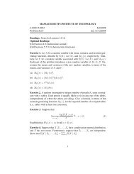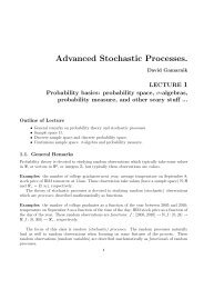
Lecture I - MIT OpenCourseWare

MIT OpenCourseWare
http://ocw.mit.edu
16.323 Principles of Optimal Control
Spring 2008
For information about citing these materials or our Terms of Use, visit: http://ocw.mit.edu/terms.

16.323 Lecture 16
Model Predictive Control
• Allgower, F., and A. Zheng, Nonlinear Model Predictive Control, Springer-Verlag,
2000.
• Camacho, E., and C. Bordons, Model Predictive Control, Springer-Verlag, 1999.
• Kouvaritakis, B., and M. Cannon, Non-Linear Predictive Control: Theory &
Practice, IEE Publishing, 2001.
• Maciejowski, J., Predictive Control with Constraints, Pearson Education POD,
2002.
• Rossiter, J. A., Model-Based Predictive Control: A Practical Approach, CRC
Press, 2003.

Spr 2008 16.323 16–1
MPC
• Planning in Lecture 8 was effectively “open-loop”
– Designed the control input sequence u(t) using an assumed model
and set of constraints.
– Issue is that with modeling error and/or disturbances, these inputs
will not necessarily generate the desired system response.
• Need a “closed-loop” strategy to compensate for these errors.
– Approach called Model Predictive Control
– Also known as receding horizon control
• Basic strategy:
– At time k, use knowledge of the system model to design an input
sequence
u(k|k), u(k + 1|k), u(k + 2|k), u(k + 3|k), . . . , u(k + N|k)
over a finite horizon N from the current state x(k)
– Implement a fraction of that input sequence, usually just first step.
– Repeat for time k + 1 at state x(k + 1)
Reference
"Optimal" future outputs
Future outputs, no control
Old outputs
Old inputs
"Optimal" future inputs
Future inputs, no control
Past Present Future Time
MPC: basic idea (from Bo Wahlberg)
Figure by MIT OpenCourseWare.
June 18, 2008

Spr 2008 16.323 16–2
• Note that the control algorithm is based on numerically solving an
optimization problem at each step
– Typically a constrained optimization
• Main advantage of MPC:
– Explicitly accounts for system constraints.
Doesn’t just design a controller to keep the system away from
them.
– Can easily handle nonlinear and time-varying plant dynamics, since
the controller is explicitly a function of the model that can be modified
in real-time (and plan time)
• Many commercial applications that date back to the early 1970’s, see
http://www.che.utexas.edu/~qin/cpcv/cpcv14.html
– Much of this work was in process control - very nonlinear dynamics,
but not particularly fast.
• As computer speed has increased, there has been renewed interest in
applying this approach to applications with faster time-scale: trajectory
design for aerospace systems.
Ref
Trajectory
Generation
u d
xd
Noise u
du
P
Plant
Feedback
Compensation
Output
Ref
Trajectory
Generation
Noise
u
P
Plant
Output
Implementation architectures for MPC (from Mark Milam)
Figure by MIT OpenCourseWare.
June 18, 2008

Basic Formulation
Spr 2008 16.323 16–3
• Given a set of plant dynamics (assume linear for now)
and a cost function
x(k + 1) = Ax(k) + Bu(k)
z(k) = Cx(k)
N
J = {z(k + j|k) Rzz + u(k + j|k) Ruu } + F (x(k + N|k))
j=0
– z(k + j|k) Rxx is just a short hand for a weighted norm of the
state, and to be consistent with earlier work, would take
z(k + j|k) Rzz = z(k + j|k) T R zz z(k + j|k)
– F (x(k + N|k)) is a terminal cost function
• Note that if N → ∞, and there are no additional constraints on z or
u, then this is just the discrete LQR problem solved on page 3–14.
– Note that the original LQR result could have been written as just
an input control sequence (feedforward), but we choose to write
it as a linear state feedback.
– In the nominal case, there is no difference between these two implementation
approaches (feedforward and feedback)
– But with modeling errors and disturbances, the state feedback form
is much less sensitive.
⇒ This is the main reason for using feedback.
• Issue: When limits on x and u are added, we can no longer find the
general solution in analytic form ⇒ must solve it numerically.
June 18, 2008

Spr 2008 16.323 16–4
• However, solving for a very long input sequence:
– Does not make sense if one expects that the model is wrong and/or
there are disturbances, because it is unlikely that the end of the
plan will be implemented (a new one will be made by then)
– Longer plans have more degrees of freedom and take much longer
to compute.
• Typically design using a small N ⇒ short plan that does not necessarily
achieve all of the goals.
– Classical hard question is how large should N be?
– If plan doesn’t reach the goal, then must develop an estimate of the
remaining cost-to-go
• Typical problem statement: for finite N (F = 0)
s.t.
N
min J = {z(k + j| k) Rzz + u(k + j|
k) Ruu }
u
j=0
x(k + j + 1|k) = Ax(k + j|k) + Bu(k + j|k)
x(k|k) ≡ x(k)
z(k + j|k) = Cx(k + j|k)
and
|u(k + j|k)| ≤ u m
June 18, 2008

Spr 2008 16.323 16–5
• Consider converting this into a more standard optimization problem.
z(k|k) = Cx(k|k)
z(k + 1|k) = Cx(k + 1|k) = C(Ax(k|k) + Bu(k|k))
= CAx(k|k) + CBu(k|k)
z(k + 2|k) = Cx(k + 2|k)
= C(Ax(k + 1|k) + Bu(k + 1|k))
= CA(Ax(k|k) + Bu(k|k)) + CBu(k + 1|k)
= CA 2 x(k|k) + CABu(k|k) + CBu(k + 1|k)
.
z(k + N|k) = CA N x(k|k) + CA N−1 Bu(k|k) + · · ·
+CBu(k + (N − 1)|k)
• Combine these equations into the following:
⎡
⎤ ⎡ ⎤
z(k|
k)
C
z(k + 1|
k)
CA
z(k + 2 | k)
=
CA 2
x(k|k)
⎢
⎥ ⎢ ⎥
⎣ . ⎦ ⎣
. ⎦
z(k + N|k) CA N
⎡
⎤
0 0 0 · · · 0 ⎡
CB 0 0 0
u(k|k)
u(k + 1|k)
+ CAB CB 0 0
⎢
⎢
⎥ ⎣ .
⎣ .
⎦
CA N−1 B CA N−2 B CA N−3 u(k + N − 1|k)
B · · · CB
⎤
⎥
⎦
June 18, 2008

Spr 2008 16.323 16–6
• Now define
⎡ ⎤ ⎡ ⎤
z(k k) u(k k)
Z(k) ≡ ⎣ . | ⎦ U(k) ≡ ⎣ . | ⎦
z(k + N|k)
u(k + N − 1|k)
then, with x(k|k) = x(k)
• Note that
Z(k) = Gx(k) + HU(k)
N
z(k + j|k) T R zz z(k + j|k) = Z(k) T W 1 Z(k)
j=0
with an obvious definition of the weighting matrix W 1
• Thus
Z(k) T W 1 Z(k) + U(k) T W 2 U(k)
= (Gx(k) + HU(k)) T W 1 (Gx(k) + HU(k)) + U(k) T W 2 U(k)
1
= x(k) T H 1 x(k) + H T 2 U(k) + U(k) T H 3 U(k)
2
where
H 1 = G T W 1 G, H 2 = 2(x(k) T G T W 1 H), H 3 = 2(H T W 1 H + W 2 )
• Then the MPC problem can be written as:
min J˜ = H T 2 U(k) + 1 U(k) T H 3 U(k)
U(k) 2
I
s.t.
N
U(k) ≤ u
−I m
N
June 18, 2008

Spr 2008
Toolboxes
16.323 16–7
• Key point: the MPC problem is now in the form of a standard
quadratic program for which standard and efficient codes exist.
QUADPROG Quadratic programming. %
X=QUADPROG(H,f,A,b) attempts to solve the %
quadratic programming problem:
min 0.5*x’*H*x + f’*x subject to: A*x

MPC Observations
Spr 2008 16.323 16–8
• Current form assumes that full state is available - can hookup with an
estimator
• Current form assumes that we can sense and apply corresponding control
immediately
– With most control systems, that is usually a reasonably safe assumption
– Given that we must re-run the optimization, probably need to account
for this computational delay - different form of the discrete
model - see F&P (chapter 2)
• If the constraints are not active, then the solution to the QP is that
U(K) = −H −1 H 2 3
which can be written as:
u(k|k) = − 1 0 . . . 0 (H T W 1 H + W 2 ) −1 H T W 1 Gx(k)
= −Kx(k)
which is just a state feedback controller.
– Can apply this gain to the system and check the eigenvalues.
June 18, 2008

Spr 2008 16.323 16–9
• What can we say about the stability of MPC when the constraints are
active? 33
– Depends a lot on the terminal cost and the terminal constraints. 34
• Classic result: 35 Consider a MPC algorithm for a linear system with
constraints. Assume that there are terminal constraints:
– x(k + N|k) = 0 for predicted state x
– u(k + N|k) = 0 for computed future control u
Then if the optimization problem is feasible at time k, x = 0 is stable.
Proof: Can use the performance index J as a Lyapunov function.
– Assume there exists a feasible solution at time k and cost J k
– Can use that solution to develop a feasible candidate at time k + 1,
by simply adding u(k + N + 1) = 0 and x(k + N + 1) = 0.
– Key point: can estimate the candidate controller performance
J˜k+1 = J k − {z(k|k) Rzz + u(k|k) Ruu }
≤ J k − {z(k|k) Rzz }
– This candidate is suboptimal for the MPC algorithm, hence J decreases
even faster J k+1 ≤ J˜ k+1
– Which says that J decreases if the state cost is non-zero (observability
assumptions) ⇒ but J is lower bounded by zero.
• Mayne et al. [2000] provides excellent review of other strategies for
proving stability – different terminal cost and constraint sets
33 “Tutorial: model predictive control technology,” Rawlings, J.B. American Control Conference, 1999. pp. 662-676
34 Mayne, D.Q., J.B. Rawlings, C.V. Rao and P.O.M. Scokaert, ”Constrained Model Predictive Control: Stability and Optimality,”
Automatica, 36, 789-814 (2000).
35 A. Bemporad, L. Chisci, E. Mosca: ”On the stabilizing property of SIORHC”, Automatica, vol. 30, n. 12, pp. 2013-2015, 1994.
June 18, 2008

Spr 2008
Example: Helicopter
16.323 16–10
• Consider a system similar to the Quansar helicopter 36
θ p
θ e
θ r
Figure by MIT OpenCourseWare.
• There are 2 control inputs – voltage to each fan V f , V b
• A simple dynamics model is that:
¨ θ e = K 1 (V f + V b ) − T g /J e
¨ θ r = −K 2 sin(θ p )
¨ θ p = K 3 (V f − V b )
and there are physical limits on the elevation and pitch:
−0.5 ≤ θ e ≤ 0.6 − 1 ≤ θ p ≤ 1
• Model can be linearized and then discretized T s = 0.2sec.
12
10
8
6
State
Control
Time
4
2
0
0 5 10 15 20 25
N
Figure 16.3: Response Summary
36 ISSN 02805316 ISRN LUTFD2/TFRT- -7613- -SE MPCtools 1.0 Reference Manual Johan Akesson Department of Automatic
Control Lund Institute of Technology January 2006
June 18, 2008

Spr 2008
0.4
0.3
4
3
16.323 16–11
Elevation [rad]
0.2
0.1
Rotation [rad]
2
1
0
0
−0.1
0 10 20 30
−1
0 10 20 30
Pitch [rad]
1
0.5
0
−0.5
−1
0 10 20 30
t [s]
V f
, V b
[V]
4
3
2
1
0
−1
−2
0 10 20 30
t [s]
0.4
0.3
Figure 16.4: Response with N = 3
4
3
Elevation [rad]
0.2
0.1
Rotation [rad]
2
1
0
0
−0.1
0 10 20 30
−1
0 10 20 30
Pitch [rad]
1
0.5
0
−0.5
−1
0 10 20 30
t [s]
V f
, V b
[V]
4
3
2
1
0
−1
−2
0 10 20 30
t [s]
0.4
0.3
Figure 16.5: Response with N = 10
4
3
Elevation [rad]
0.2
0.1
Rotation [rad]
2
1
0
0
−0.1
0 10 20 30
−1
0 10 20 30
Pitch [rad]
1
0.5
0
−0.5
−1
0 10 20 30
t [s]
V f
, V b
[V]
4
3
2
1
0
−1
−2
0 10 20 30
t [s]
June 18, 2008
Figure 16.6: Response with N = 25