Crystal Structure 1 3.1 Some Basic Concepts of Crystal Structure ...

Crystal Structure 

Basic Concepts 

3.1 Some Basic Concepts of Crystal Structure: Basis and Lattice 

A crystal lattice can always be constructed by the repetition of a fundamental set of 

translational vectors in real space a, b, and c, i.e., any point in the lattice can be written 

as: 

r = n 1 a + n 2 b + n 3 c. (3.1) 

Such a lattice is called a Bravais lattice. The translational vectors, a, b, and c are the 

primitive vectors. Note that the choice for the set of primitive vectors for any given 

Bravais lattice is not unique. 

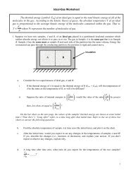
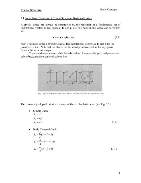
There are three common cubic Bravais lattices: Simple cubic (sc), body-centered 

cubic (bcc), and face-centered cubic (fcc). 

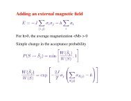
Fig. 3.1 (from Kittle) The cubic space lattices. The cells shown are the conventional cells. 

The commonly adopted primitive vectors of these cubic lattices are (see Fig. 3.2): 

 

 

Simple Cubic 

 

a1 

ax 

a 

ayˆ 

2 

a 

azˆ 

3 

Body Centered Cubic 

a 

a ( ˆ 

1 

x y zˆ) 

2 

a 

a ( ˆ 

2 

x 

y zˆ) 

2 

a 

a ( ˆ 

3 

x y zˆ) 

2 

(3.2) 

(3.3) 

1



 

Face Centered Cubic 

 

a1 a( 

x yˆ) 

 

a ( ˆ 

2 

a y zˆ) 

 

a a( 

x ˆ) 

3 

z 

(3.4) 

(a) 

(b) 

Fig. 3.2 

Coordination number: The points in a Bravais lattice that are closest to a given point are 

called its nearest neighbors. Because of the periodic nature of a Bravais lattice, each point 

has the same number of nearest neighbors. This number is called the coordination 

number. For example, a sc lattice has coordination number 6; a bcc lattice, 8; a fcc lattice, 

12. 

Primitive unit cell: A volume in space, when translated through all the lattice vectors in a 

Bravais lattice, fills the entire space without voids or overlapping itself, is a primitive unit 

cell (see Figs. 3.3 and 3.4). Like primitive vectors, the choice of primitive unit cell is not 

unique (Fig. 3.3). It can be shown that each primitive unit cell contains precisely one 

lattice point unless it is so chosen that there are lattice points lying on its surface. It then 

follows that the volume of all primitive cells of a given Bravais lattice is the same. 

2



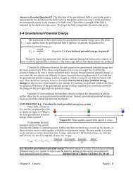
Fig. 3.3 (from A&M) Several possible choices of primitive cell for the 

same two-dimensional Bravais lattice. 

(a) 

(b) 

Fig. 3.4 (from A&M) Primitive unit cell for the choice of primitive vectors specified in Eqs. 3.3 and 3.4 

for, respectively, an (a) fcc and (b) a bcc Bravais lattice. 

Unit cell and lattice constants: A unit cell is a volume, when translated through some 

subset of the vectors of a Bravais lattice, can fill up the whole space without voids or 

overlapping with itself. The conventional unit cell chosen is usually bigger than the 

primitive cell in favor of preserving the symmetry of the Bravais lattice. For example, the 

primitive cells shown in Figs. 3.4(a) and (b) for respectively the fcc and bbc Bravais 

lattice are parallelipipeds that do not bear the cubic symmetry of their own lattice. The 

conventional unit cell of the respective lattice is the cubic cell shown in the same figure. 

Note that the volume of the conventional unit cell is four times that of the primitive unit 

cell for fcc, and two times for bcc. The lattice constant, a, of a cubic lattice (sc, bcc and 

fcc) refers to the length of the side of the cubic unit cell. 

3



Wigner-Seitz primitive cell: It turns out one can always choose a primitive unit cell with 

the full symmetry of the Bravais lattice. The most popular choice is the Wigner-Seitz cell. 

By construction, there is only one Wigner-Seitz cell about a lattice point. To construct a 

Wigner-Seitz cell, one draws lines connecting one given lattice point to all its nearby 

points in the lattice, bisects each line with a plane, and takes the smallest polyhedron 

containing the point bounded by these planes. Fig. 3.5 illustrates the Wigner-Seitz cell of 

a two-dimensional Bravais lattice. Figs. 3.6 and 3.7 illustrate the Wigner-Seitz cell for the 

bbc and fcc lattice, respectively. 

Fig. 3.5 (from (A&M) The Wigner-Seitz cell of 

a two-dimensional Bravais lattice. 

Fig. 3.6 (from A&M) The Wigner-Seitz cell for 

the bcc Bravais lattice (a “truncated 

octahedron”). The surrounding cube is a 

conventional bcc cell with a lattice point at its 

center and on each vertex. The hexagonal faces 

bisect the lines joining the central point to the 

points on the vertices (drawn as solid lines). 

The square faces bisect the lines joining the 

central point to the central points in each of the 

six neighboring cubic cells (not drawn). 

Fig. 3.7 (from A&M) The Wigner-Seitz cell for 

the fcc Bravais lattice (a “rhombic 

dodecahedron”). The surrounding cube is not 

the conventional bcc cell of Fig. 3.4(a), but one 

in which lattice points are at the center of the 

cube and at the center of the 12 edges. Each of 

the 12 faces (all identical in shape and size) is 

perpendicular to a line joining the central point 

to a point on the center of an edge. 

4




In the above, we have discussed the concept of crystal lattice. To complete a crystal 

structure, one needs to attach the basis (a fixed group of atoms) to each lattice point, i.e., 

Bravais Lattice + Basis = Crystal Structure 

Fig. 3.8 (From Kittel) The crystal 

structure is formed by the addition of the 

basis (b) to the lattice points of the lattice 

(a). By looking at (c), you can recognize 

the basis and then you can abstract the 

space lattice. It does not matter where the 

basis is put in relation to a lattice point. 

Some examples: 

(1) Diamond structure 

Fig. 3.9 (From A&M) Conventional cubic cell of 

the diamond lattice. This structure consists of two 

interpenetrating fcc lattices, displaced along the 

body diagonal of the cubic cell by ¼ the length of 

the diagonal. It can be regarded as a fcc lattice 

with the two-point basis at (000) and 1/4(111). 

Note that the diamond structure is not a Bravais 

lattice. 

5



(2) Sodium chloride structure 

Fig. 3.10 (From Kittel) The sodium chloride 

structure is produced by arranging Na + and Cl 

ions alternatively at the lattice points of a sc 

lattice. In the crystal each ion is surrounded by 6 

nearest neighbors of the opposite charge. The 

space lattice is fcc, and the basis has one Na + at 

½(111) and Cl at (000). The figure shows one 

conventional unit cell. The ionic diameters here 

are reduced in relation to the cell in order to 

clarify the spatial arrangement. 

(3) Hexagonal close-packed (hcp) structure 

A hexagonal closed-packed structure is built upon two simple hexagonal Bravais 

lattices. Figure 3.11 shows a simple hexagonal Bravais lattice. Figure 3.12 shows the 

structure of a hcp, and how it is constructed from two simple hexagonal structures. 

Fig. 3.11 (From A&M) A simple hexagonal Bravais lattice (a) in 3-dimensions (b) in 2-dimensions. 

6


Bragg Diffraction & Reciprocal Lattice Vectors 

Fig. 3.12 (From A&M) The hcp structure. It can 

be viewed as two interpenetrating simple 

hexagonal lattices, displaced vertically by a 

distance c/2 along the common c-axis, and 

displaced horizontally so that the points of one lie 

directly above the centers of the triangles formed 

by the points of the other. 

3.2 Bragg Diffraction and Reciprocal Lattice Vectors 

Bragg Diffraction (Simple Picture) 

Periodic lattice planes 

Fig. 3.13 Schematic diagram illustrating the condition for Bragg diffraction. 

Bragg diffraction condition: 

2d sin = n 

 

where n = 1, 2, 3, … (3.5) 

7


Bragg Diffraction and Reciprocal Lattice Vectors 

An incident beam of radiation or particles is diffracted from a crystal only if the Bragg 

diffraction condition (3.5) is satisfied. We can view it as the condition where 

constructive interference takes place between the diffracted radiation or particles from the 

adjacent planes. Since the lattice constant of crystals is of the order of 2 to 3 Å, for easily 

measurable (such as ~1 to 10 o ) at the first order Bragg diffraction, it is desirable for the 

wavelength of the beam, ~ 0.1 to 1Å. These values correspond to the wavelength of x- 

rays and 10 - 100 keV electrons. The latter constitutes the basics of transmission electron 

microscopes. 

Miller Indices 

Miller indices are convenient labels of crystal planes. The following are steps to 

determine the Miller indices of a crystal plane: 

(1) Determine the intercepts l 1 , l 2 and l 3 of the plane on the three translation axes in 

units of the translation vectors. 

(2) Take the reciprocal of the intercepts (1/l 1 , 1/l 2 1/l 3 ) and multiple by the smallest 

constant that makes them integers (h, k, l). 

Miller Indices can also be used to label the group of equivalent planes {h, k, l}. 

Examples: 

(2, 3, 3) 

Fig. 3.14 

8




Reciprocal Vectors 

The reciprocal lattice of a Bravais lattice constructed by the set of primitive vectors, a, b 

and c is one that has primitive vectors given by: 

 

 

 

b c 

 

c a 

 

a b 

A 2 B 2 C 

a b c 

a b c 

2 

a b c 

(3.6) 

Examples: 

(1) Reciprocal lattice to simple cubic lattice 

For sc lattice, we may choose the following set of primitive vectors: 

 

a aˆ, 

a aˆ, 

a aˆ, 

1 

x 

2 

y 

3 

z 

We may then determine the reciprocal lattice vectors b 1 , b 2 and b 3 using eqn. 3.6: 

 

 

a2 

a3 

2 

b 2 xˆ 

1 

. 

3 

a a 

Similarly, 

2 

2 

b yˆ 

2 

and b3 

zˆ 

a 

a 

9



10


Next we discuss the physical meaning of reciprocal lattice vectors as defined in eqn. 3.6. 

Consider the primitive vectors, a, b and c of a lattice as depicted below. 

We first focus on the plane (100) as marked in the figure. One may observe that the area 

of this plane is |a b| and the cross product a b is normal to the plane and directed 

away from the origin. In addition, the volume of the parallelepiped generated by a, b and 

c, which we label by V abc is a (b c) (= b (c a) = c (a b)). It follows that the 

distance between this plane the one next and parallel to it is: 

 

Vabc 

a b c 

d100 . 

b c b c 

(3.7) 

Therefore, the reciprocal lattice vector, A, as defined in eqn. 3.6 can be rewritten as: 

 

 

 

b c 1 

A 2 

2 

nˆ 

100 

d 

(3.8) 

a b c 

100 

where n 100 is the unit vector normal to (100) (and directed away from the origin.) By 

repeating the argument for the other two planes, i.e., (010) and (001), we have: 

 

B 

 

C 

1 

2 

nˆ 

d 

010 

1 

2 

nˆ 

d 

001 

010 

001 

(3.9) 

where n 010 and n 001 is the unit normal to (010) and (001), respectively. 

11


The above result can be generalized to an arbitrary reciprocal lattice vector, G = hA + kB 

+ lC. In other words, G is related to the plane (h k l) by the following relations: 

(1) G is normal to the plane (h k l). 

(2) The distance d hkl between adjacent planes with the Miller indexes (h k l) is given 

by 2/|G|. 

Proof: 

(1) By definition, a plane (h k l) intersects the 

crystallographic axes along a, b and c at the points 

l 1 a, l 2 b and l 3 c, respectively, where 

l1 : l2 

: l3 

 

1 1 1 

: : 

h k l 

where l 1 , l 2 and l 3 are integers. Now, all planes whose 

intercepts fulfill the above relation are parallel. 

Therefore, it suffices to prove that the one plane with intercepts 1/h, 1/k and 1/l is 

perpendicular to G. One may observe that any vector on this plane can be expressed as a 

linear combination of the vectors (1/h)a – (1/k)b, (1/k)b – (1/l)c and (1/l)c – (1/h)a. It 

follows that if G is perpendicular to all of these three vectors, G must be parallel to (h k 

l). As shown below, this is indeed the case. 

Note that this proof works only if none of h, k or l is zero. Suppose l = 0. Then the plane 

to be considered is spanned by (1/h)a – (1/k)b and c. It is straightforward to show that hA 

+ kB is perpendicular to these two vectors. In the case where two of the Miller indices 

are zero, say k = l = 0, G = A. We have shown above that it is perpendicular to the (1 0 0) 

plane (eqn. 3.8). 

12



We now return to Bragg diffraction and see how it is related to the reciprocal lattice 

vectors. Recall eqn. (3.5) for the Bragg diffraction condition: 

2d sin = n 

 

where n = 1, 2, 3, … 

Experimentally, it is found that Bragg diffraction is elastic, i.e., the energy of the 

incoming beam is equal to that of the outgoing beam. For x-ray, E = ħ = ħ|k|c, where c 

is speed of light and k is the wavevector of the incident x-ray. Elastic scattering means 

that |k| =| k’|, where k’ is the wavector of the outgoing x-ray beam. Given this, one may 

construct the following vector diagram: 

13


The vector, k = k’ – k is the change in wavevector and proportional to the change in 

momentum of the x-ray upon diffraction. At the first order diffraction, 

2d sin = k 

2k sind = |G|, (3.10) 

where G is the reciprocal lattice vector associated with the diffraction planes. It is also 

evident from the above figure that k is perpendicular to the diffraction planes. In order 

words, k is parallel to G. Combining this with eqn. (3.10) we have: 

k = G 

(3.10b) 

Eqn. 3.7 states the important fact that a (photon or particle) beam diffracted by the Bragg 

plane (h k l) always suffers a change of momentum equals G = hA + kB + lC in both 

magnitude and direction. With this, we may discuss the Ewald construction. 

Ewald Construction 

Ewald construction provides a convenient graphical method to look for the Bragg 

diffraction condition for a Bravais lattice. The procedure is as the following: We draw in 

reciprocal space a sphere centerd on the tip of the incident wavevector k (drawn from the 

origin) of radius k. This is the Ewald sphere. A diffracted beam will form if this sphere 

intersects any lattice point, K, in the reciprocal space. The direction of the diffracted 

beam is the direction of k’ ( k K). 

14



(from A&M) 

The Ewald construction may help us understand the principle of some common x-ray 

diffraction techniques used for the determination of crystal structures. 

Laue Diffraction Method 

This method is widely used for quick determination of the orientation of a crystal 

surface. The experimental setup is shown in Fig. 3.19. During the measurement, the 

sample is kept stationary, and is irradiated by a well-collimated x-ray beam with a broad 

spectral distribution. Both the forward and backward scattered rays are recorded on 

photographic films. The resulting pattern is a set of points (which are the diffraction 

spots), each coming from one set of crystallographic planes. The Ewald construction of 

Fig. 3.21 illustrates the principle. 


15


Fig. 3.20 Laue pattern of a Si crystal in approximately the [100] direction. 

Fig. 3.21 The Ewald construction for the Laue 

method. The crystal and incident x-ray direction are 

fixed, and a continuous range of wavelengths, 

corresponding to wavevectors between k 0 and k 1 in 

magnitude is present. The Ewald spheres for all 

incident wavevectors fill the shaded region between 

the sphere centered on the tip of the vector k 0 and that 

centered on the tip k 0 . Bragg peaks will be observed 

corresponding to all reciprocal lattice points lying 

within the shaded region. (For simplicity in 

illustration, the incident direction has been taken to lie 

in a lattice plane, and only reciprocal lattice points 

lying in that plane are shown. (from A&M) 

16


Rotating Crystal Method 

This method uses a monochromatic beam of x-ray from a source that is fixed. The 

incident angle, , is variable by rotating the crystal orientation. (Note that is the angle 

between the incident x-ray and the crystal plane, not the sample surface (Fig. 3.23)) The 

detector is moved (by rotating the detector arm) to intercept the diffracted beam. Once 

the diffracted beam is found, is determined to be a half of the angle between the 

incident x-ray and the detector orientation, in accordance to the Bragg diffraction law. 

The single crystal is rotated by a precision goniometer to bring sets of atomic planes into 

positions for the Bragg diffraction during the measurement. The axis of rotation of the 

detector arm is perpendicular to both the incident and reflected beams. A diffraction spot 

is detected when a set of crystal planes with the appropriate inter-planar separation, d, 

satisfies the Bragg condition. The Ewald construction of Fig. 3.23 illustrates the principle 

of operation. 

To detector 

(rotatable) 

 

collimator 

 

2 

collimator 

Sample (rotatable) 

Fig. 3.22 Schematic diagram for the setup of the rotating crystal method. 

Fig. 3.23 The Ewald construction for the 

rotating-crystal method. For simplicity a case is 

shown in which the incident wavevector lies in a 

lattice plane. The concentric circles are the orbits 

swept out under the rotation by the reciprocal 

lattice vectors lying in the plane perpendicular to 

the axis containing k. Each intersection of such a 

circle with the Ewald sphere gives the 

wavevector of a Bragg reflected ray. 

(Additional) Bragg reflected wavevectors 

associated with reciprocal lattice vectors in other 

planes are not shown. (From A&M) 

17


Powder Diffraction 

In this method, the specimen is in a powder form hence contains a large number of 

crystallites in random orientation. The x-ray used is monochromatic. Fig. 3.24 shows the 

schematic diagram of the setup and a powder diffraction pattern from ZnO. A set of 

atomic planes with spacing d will give rise to a diffracted beam at an angle 2 (with 

respect to the incoming direction of the incident x-ray) according to the Bragg law. Since 

the orientation of the crystallites is random, the diffracted beam can at any azimuthal 

direction. The diffracted beams will spread around the surface of a cone with the apex at 

the specimen. 


Fig. 3.24 Schematic diagram of the setup for the powder diffraction method, and a powder pattern 

obtained from a ZnO sample. 

18


Fig. 3.25 The Ewald construction for the powder method. (a) The Ewald sphere is the smaller sphere. It is 

centered on the tip of the incident wavevector k with radius k, so that the origin 0 is on its surface. The 

larger sphere is centered on the origin and has a radius K. The two spheres intersect in a circle 

(foreshortened to an ellipse). Bragg reflections will occur for any wavevector k’ connecting any point on 

the circle of intersection to the tip of the vector k. The scattered rays therefore lie on the cone that opens in 

the direction opposite to k. (b) A plane section of (a), containing the incident wavevector. The triangle is 

isosceles, and thus K = 2ksin(/2). 

19


3.3 Kinematic Theory of Scattering 

r 

dV 

 

k 

k’ 

Incident beam 

e ik·r 

kr 

|k| 

k’r 

|k’| 

Outgoing beam 

e ik’·r 

r 

k 

k’ 

Fig. 3.26 

(from Kittel) 

The Bragg law only provides a condition for diffraction to occur. We need a deeper 

analysis to determine the scattering intensity from the basis of atoms. 

Consider an incoming x-ray with wavevector k. We want to calculate the 

scattering intensity in the direction along k’ due to a crystal (Fig. 3.26). First, we notice 

that waves scattered from different points of the specimen emerge with different path 

lengths from the wave scattered from the origin. For the wave scattered from a point at r, 

the path length difference between this emergent wave and that from the origin is 

(/2)(kk’)r. This leads to an extra phase factor of exp[i(kk’)r] in the wave scattered 

from point r compared to that scattered from the origin. Since the amplitude of the wave 

scattered from a volume element is proportional to the local electron concentration, n(r), 

the total amplitude of the scattered wave in the direction of k’ is proportional to the 

integral over the crystal of n(r)dV times the phase factor exp[i(kk’)r]. In other words, 

the amplitude of the electric or magnetic field vectors in the scattered electromagnetic 

wave is proportional to the following integral which defines the scattering amplitude, F: 

F = dV n(r) exp[i(kk’)r] = dV n(r) exp[ikr], (3.11) 

where k = k’ k (3.12) 

20


To evaluate the integral in eqn. 3.11, we will exploit the fact that n(r) is periodic, i.e. 

invariant under translation along any lattice vectors (which must be a linear combinations 

of the Bravais primitive vectors, a, b, and c.) Under this condition, the Fourier expansion 

of n(r) will be: 

G must be such that 

 

 

n( r ) n exp( iG r ) where (3.13) 

 

G 

G 

n(r + ma + nb + pc) = n(r) for integers m, n, p. (3.14) 

Here, n G is given by the Fourier transformation of n(r): 

n G = (1/V) dV n(r) exp[iGr] (3.15) 

Eqn. 3.15 can be shown to be consistent with eqn. 3.13. We will now show that G must 

be a reciprocal lattice vector, i.e. 

G = jA + kB + lC (3.16) 

where j, k, l are integers, and A, B, C are as defined in eqn. 3.6. Substitute eqn. 3.14 in 

eqn. 3.16, we have: 

 

 

 

n( r ) n exp( iG r ) n exp( iG r )exp[ iG ( ma nb pc)] 

n( 

r ma nb pc) 

 

 

G 

G 

Eqn. 3.17 is valid only if: 

 

 

G 

G 

(3.17) 

G(ma + nb + pc) = 2M 

 

where M is an integer. Let’s write G as a linear combination of A, B, and C, as in eqn. 

3.16, but putting no restriction on j, k, l. If we find in the end that j, k, l have to be 

integers, G must then be a reciprocal lattice vector. Substitute eqn. 3.16 in eqn. 3.18, and 

use the following relations, which are straightforward to verify: 

Then we have: 

aA = bB = cC = 2 

aB = aC = bA = bC = cA = c B = 0. (3.19) 

jm + kn + lp = M 

21


Since m, n, p, and M are integers, eqn. 3.20 can be valid in general only if j, k, l are 

integers. This proves that G must be a reciprocal lattice vector. We now go back to the 

evaluation of the integral in eqn. 3.11. Substitute eqn. 3.13 in eqn. 3.11, we have: 

F 

 

G 

dV n 

 

G 

 

exp[ i( 

G k 

) r] 

(3.21) 

= V n G (Gk) (3.22) 

The factor (Gk) provides an explanation to the Bragg diffraction law, namely k = 

GBut more informative than the Bragg diffraction law, eqn. 3.22 even tells us what the 

scattering amplitudes be for the various Bragg diffraction peak. In particular for the 

diffraction peak corresponding tok G, the scattering amplitude is just proportional to 

the G-component (n G ) in the Fourier expansion of the sample electronic distribution. 

Before we continue with the calculation of F, we will divert our discussion to the 

important concept of Bragg diffraction of electrons at a Brillouin zone boundary. 

3.31 Brillouin zone 

Brillouin zone is defined as a Wigner-Seitz primitive cell in the reciprocal lattice. 

As explained before, a Wigner-Seitz cell about a lattice point is constructed by drawing 

lines connecting the lattice point to all nearby points in the lattice, bisecting each line 

with a plane, and taking the smallest polyhedron containing the point bounded by these 

planes. With this construction, ½G must be perpendicular to and terminates at a 

Fig. 3.27 

boundary of the zone (Fig. 3.27). We will show that any wave that has wavevector, k, 

drawn from the origin and terminates at a zone boundary always satisfies the Bragg 

diffraction condition hence will be Bragg diffracted. From Fig. 3.27, it is obvious that 

 

k ( G 

(3.23) 

1 1 2 

2 G) 

( ) 2 

22


According to eqn.10, the Bragg law is equivalent to: 

2k 

sin 

G 

 

G 

2k 

G 

G 

 

2 

2k 

G 

G 

 

k ( G) 

( 

1 

2 

1 

2 

 

G) 

2 

which is the same as eqn. 3.23. This proves our proposition. Since this conclusion is 

general to all kinds of waves, it is valid in particular to electron waves traversing in the 

crystal. This result says that electrons with wavevector k reaching a Brillouin zone 

boundary will suffer strong Bragg diffraction by the crystal planes. 

3.32 Structure Factor and Form Factor 

Let’s now come back to the evaluation of the scattering amplitude F from eqn. 

3.22. Substitute eqn. 3.15 in eqn. 3.22: 

F = V n G (Gk) 

= dV n(r) exp[ik r] 

If N is the total number of unit cells in the solid, and because the crystal is periodic, 

F = N unit cell dV n(r) exp[ik r] (3.24) 

= N S G 

where S G is called the structure factor. Note that it is an integral over a unit cell, with r = 

0 at one corner. It is often convenient to write the electron concentration as the 

superposition of electron concentration functions, n j associated with each atom j in the 

basis. If r j is the position vector of the atom j in the basis, our proposition means that 

s 

n( 

r ) 

n ( r r ) , (3.25) 

where s is the total number of atoms in a cell. Note that the expansion of n(r) in the form 

of eqn. 3.25 is not unique. Particularly, it is not possible to distinguish how much charge 

is associated with each atom. But this in general is not a problem. 

S 

G 

 

 

s 

j1 

s 

 

j1 

j 1 

j 

j 

 

dVn 

j 

( r rj 

)exp( ik 

r ) 

 

exp( ik 

r ) dVn ( 

)exp( ik 

 

) , (3.26) 

where is defined as r r j . We now defined the atomic form factor as: 

j 

 

j 

23


 

f 

j 

dVn 

j 

( )exp( ik 

 

). 

(3.27) 

Substitute eqn. 3.27 in eqn. 3.26: 

S 

G 

 

s 

j 1 

 

exp( ik 

r ) f 

j 

j 

(3.28) 

Suppose, k = mA + nB + pC, (m, n, p integers) and r j = x j a + y j b + z j c (x, y, z real 

numbers). 

Hence, eqn. 3.28 can be rewritten as: 

kr = 2(mx j + ny j + pz j ) (3.29) 

S 

G 

s 

j 1 

( m, 

n, 

p) 

f exp( i2 ( mx ny pz ) (3.30) 

j 

j 

j 

j 

Examples 

(1) Structure factor of bcc lattice 

The bcc basis referred to the cubic cell has identical atoms at r 1 = (0,0,0) and r 2 = 

1/2(1,1,1). Hence, 

S G (m, n, p) = f[1 + exp(i(m + n + p))] (3.31) 

Since exp(iN) = 1 if N is even, but = 1 if N is odd, 

S G (m, n, p) = 2f if m + n + p is even 

= 0 if m + n + p is odd. (3.32) 

Eqn. 3.32 points out that the diffraction spectrum of bcc solids do not containing lines 

such as (100), (300), (111), etc. The physical origin for the absence of these lines can be 

understood with the help of Fig. 3.28. As seen, there is an intervening plane (200) 

between any two adjacent (100) planes. When the Bragg condition is satisfied for the 

(100) planes, reflections from adjacent planes differ by a phase of exactly 2. The 

intervening (200) plane, on the other hand, produces a reflection retarded in phase by 

with respect to the first plane, thereby canceling the contribution from that plane. 

24


Fig. 3.28 Explanation of the absence of a (100) reflection from a bcc lattice. The phase difference between 

successive planes is , so that the reflected amplitude from two adjacent planes is 0. 

(2) Structure factor of fcc lattice 

The basis referred to the cubic cell has identical atoms at 000; 0½½; ½0½; ½½0. 

Hence, 

S G (m, n, p) = f{1 + exp[i( n + p)] + exp[i(m + p)] + exp[i(m + n)]} (3.31) 

There are 4 cases: 

1. All m, n, p are even. Then S G (m, n, p) = 4. 

2. All m, n, p are odd. We have the same result as in 1. 

3. Two of the m, n, p are even. Then one of the exponentials is +1 and two of the 

exponentials are –1. Hence S G (m, n, p) = 0. 

4. Two of the m, n, p are odd. We have the same result as in 3. 

Hence, in fcc, no reflection can occur for those with indices that are partly even, or partly 

odd. (see Fig. 3.29 for the comparison between the scattering spectrum of KCl and that of 

KBr.) 

Effect of form factor on the diffraction spectrum 

 

From eqn. 3.27, atomic form factor, f 

j 

dVn 

j 

( )exp( ik 

 

). This shows that it is 

essentially the Fourier transformation of the electron distribution about the atom at r j . We 

can think of how qualitatively f j should vary with the spatial extent of the electron 

distribution. In the limit where the charge is concentrated at one point, the Fourier 

transformation (hence f) will be flat in k-space. But if the charge distribution is smeared 

out, f will be decreasing from k = 0 with width of the order equal the reciprocal of the 

size of the charge distribution. 

25


Fig. 3.29 

sin 

Fig. 3.30 Experimental atomic scattering factors for metallic aluminum. (from Kittel) 

26

Crystal Structure 1 3.1 Some Basic Concepts of Crystal Structure ...

You also want an ePaper? Increase the reach of your titles

Delete template?

Save as template?