Introduction to Unconstrained Optimization - Scilab

0
0
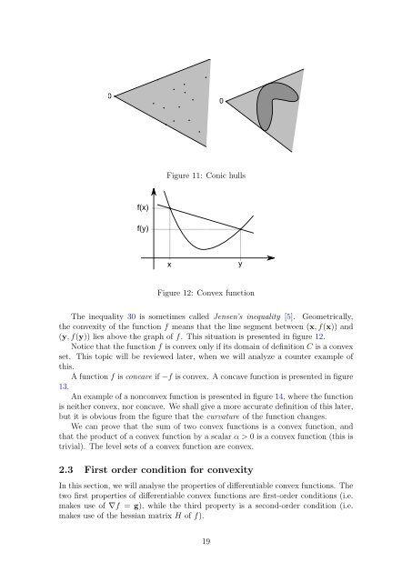
Figure 11: Conic hulls
f(x)
f(y)
x
y
Figure 12: Convex function
The inequality 30 is sometimes called Jensen’s inequality [5]. Geometrically,
the convexity of the function f means that the line segment between (x, f(x)) and
(y, f(y)) lies above the graph of f. This situation is presented in figure 12.
Notice that the function f is convex only if its domain of definition C is a convex
set. This topic will be reviewed later, when we will analyze a counter example of
this.
A function f is concave if −f is convex. A concave function is presented in figure
13.
An example of a nonconvex function is presented in figure 14, where the function
is neither convex, nor concave. We shall give a more accurate definition of this later,
but it is obvious from the figure that the curvature of the function changes.
We can prove that the sum of two convex functions is a convex function, and
that the product of a convex function by a scalar α > 0 is a convex function (this is
trivial). The level sets of a convex function are convex.
2.3 First order condition for convexity
In this section, we will analyse the properties of differentiable convex functions. The
two first properties of differentiable convex functions are first-order conditions (i.e.
makes use of ∇f = g), while the third property is a second-order condition (i.e.
makes use of the hessian matrix H of f).
19