Logic of Significance Tests - ncssm

Introducing the Logic of Significance Testing through Simulation 

The following activities are designed with a few objectives in mind: 

1. To develop the skills necessary to design and conduct a simulation 

2. To informally introduce the idea of a sampling distribution 

3. To informally introduce the logic of significance testing 

Simulations can (and should) be used throughout an AP Statistics course. Likewise, the 

idea of inference should be present throughout the course. The activities that follow are 

intended to be introductions to simulations, sampling distributions, and significance tests. 

They can be used as early as the first day of class or as the introduction to a unit on 

inference. They are arranged in order of increasing difficulty, however, so they should be 

done in order. The only skill necessary is the ability to graph univariate data in a dotplot 

or similar display. 

In an attempt to be consistent with our language, we will use the the following definitions 

of key terms: 

-A run is a set or collection of steps that constitute a re-enactment of the “real” 

situation and its associated outcome. (Note: a run is often called a 

repetition or a trial in other sources.) 

-A simulation is a set or collection of runs and their associated outcomes. 

In the teacher notes for each problem, three methods are proposed to execute the 

simulation: using manipulatives, using a random digit table, and using technology, 

including a graphing calculator or computer. You may use any or all of the methods for 

each problem, although we suggest that you start with manipulatives for at least the first 

problem (initially, most students have a surprisingly difficult time with the abstraction 

required for simulation). 

Simulations are most effective when a large number of runs are performed. To achieve 

this, it is beneficial to pool data from the entire class. Many teachers put an axis on the 

chalkboard or on a piece of butcher paper and allow the students to come forward and put 

an “X” above the number they got in their run. Other teachers have the students remain 

in their seats while they record the data on an overhead projector, etc. 

At the end of each problem in the teacher’s notes there are several extensions which 

include other questions or simulations relating to the same scenario. We suggest you 

read these before you introduce the problems to the students, as your decision to do one 

of the extensions might change the manner in which you record the data. 

Why use simulation to introduce the ideas of sampling distributions and significance 

tests? Traditionally, one of the hardest topics for students to understand is sampling 

distributions. Using simulation allows students to clearly see that each time they take a 

sample or perform an experiment the result they get is just one of many possible results 

and that a sampling distribution is a display of those possible results. For example, in the 

2001 NCSSM Statistics Institute 1 Dennis Holland and Josh Tabor

graph below, each “x” represents a result from one run. Thus, this distribution could 

have been made from 20 runs from 1 student, 1 run from 20 students, etc. 

x 

x x x 

x x x x x x x 

x x x x x x x x x 

1 2 3 4 5 6 7 8 9 

After forming the sampling distribution, the properties such as shape, center, and spread 

can be discussed. Also, simulations help students understand the notion of a p-value. For 

example, based on the distribution it is easy to estimate the probability of getting a result 

7 or greater (4/20). 

Finally, simulations are a great method for solving problems where the theory is difficult. 

The first problem included could easily be solved with knowledge of binomial 

distributions. The second, and especially the third are very difficult to solve theoretically. 

Yet, with simulation, the solution can be estimated in a very short period of time. 

Problems: 

1. A county is 50% African-American and 50% Caucasian and an African-American 

man is on trial. A jury has been selected that contains 8 Caucasians and 4 African- 

Americans. The defendant claims racial bias in the jury selection because its makeup 

seems unlikely given the racial percentages in the county. However, the prosecutor 

claims that the jury was selected without regard to race. Is the defendant’s claim of racial 

bias credible? In other words, is selecting 4 or fewer African-Americans unlikely to 

happen just by chance? Use a simulation to estimate the probability of selecting 4 or 

fewer African-American jurors simply by chance and use your result to analyze the 

defendant’s claim. 

2. A cereal company places a toy in every box of cereal. There are 4 different toys that 

the company claims are distributed equally in the boxes. A shopper wanted one of each 

toy for a child. She had to buy 15 boxes of cereal before she found at least one of each of 

the 4 toys. She claims that because it took her 15 boxes to find all 4 toys, the toys were 

not equally distributed. Is her claim credible? In other words, if you assume equal 

distribution of toys how unusual is it that it would take 15 or more boxes to find the 4 

different toys? Use a simulation to estimate the probability of needing to buy 15 or more 

boxes and use your results to assess her claim. 


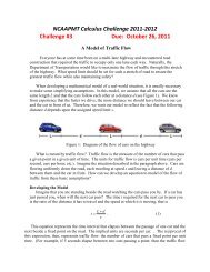
3. After a 5-hour shift watching for speeders on a rural highway, Officer Daniel Teague 

returned to his station with $600 worth of tickets. His supervisor was upset, however, 

since he thought that $600 was unusually low for such a long shift. “Stop spending so 

much time at the Donut shop!” he says. Big Dan, however, responded that he was not 

wasting time and claims it was just a slow day on the highway. 

In this state, fines are determined based on how many miles per hour the driver is 

exceeding the posted speed limit (see table below). The department policy is to pull over 

any driver going more than 10 miles per hour over the speed limit and based on past 

observations, the department has estimated what percentage of cars on the highway are 

speeding (see table below). Finally, on a typical day, a police officer will observe one car 

per minute and spend 30 minutes every time he has to stop a speeder and issue a ticket 

(no warnings in this town!). 

MPH over Speed Limit Fine Percent of Drivers 

0-10 $0 90% 

11-15 $100 7% 

16-20 $200 2% 

20 or more $300 1% 

Was the supervisor too harsh, or was Big Dan Teague telling the truth? Conduct a 

simulation to estimate the probability of issuing $600 or less in speeding tickets in a 5 

hour (300 minute) shift given the information above. 

Note: Occasionally an officer will have to give a ticket during the last 30 minutes of his 

shift. In this case, he will still give the ticket, even though it means he will be on duty for 

more than 300 minutes. For example, if he finds a speeder during minute 299, he will be 

on duty until minute 329. 


Teacher’s Notes 

Problem 1: 

A. Possible methods using manipulatives: 

Because there are two equally likely outcomes from the population, it is 

possible to simulate the selection of each juror by one coin flip. Assign 

Heads=African-American and Tails=Caucasian. To complete a single run, 

flip the coin 12 times and record the number of African-Americans (number 

of Heads). 

It is also possible to use a spinner to simulate the selection of each juror. In 

this case, a pie chart divided into two equal sections would be both easy to 

make and easy to use. Once the chart is printed, have students un-bend one 

loop of a small paperclip to use as the pointer. Using a pencil tip at the center 

of the circle to keep the paperclip in place, flick the paperclip to spin it. (See 

the appendix for an example.) 

This simulation could also be done with red and black cards or two colors of 

beads. However, to maintain the stated model probabilities when cards are 

used, each time a juror is selected the card should be replaced and the deck 

reshuffled. If, for example, a red card is chosen and not replaced then the 

probability of a second red card is 25/51, but the probability of a black card is 

26/51. 

Similarly, with a small number of beads replace a bead when it has been 

picked or have a large number of beads to minimize the effects of a finite 

population of objects (cards, beads, etc.) used in doing the simulation. The 

rule of thumb that is commonly used is that if the sample size is less than 1/10 

of the population size the effect of drawing a sample from the finite 

population is minimal and therefore ignored. If the drawing process is done 

with replacement, there is no change in the probabilities used in each 

Bernoulli trial. 

B. Possible method using random digit table: 

Assign even digits to represent African-Americans and odd digits to represent 

Caucasians. Select 12 digits and count the number of African-Americans 

(even digits). This would complete a single run. The choice of even and odd 

digits to represent the races is arbitrary; any scheme using 5 digits for each 

will work, such as 0-4 to represent African-American and 5-9 to represent 

Caucasian. 


C. Possible method using a graphing calculator/computer: 

Assign 1 to represent the selection of an African-American and 0 to represent 

the selection of a Caucasian. Generate a list of 12 random digits that are 

either 1 or 0 and then add the digits to find the number of African-Americans. 

Using only 0 and 1 in the assignment makes it easier to count the number of 

African-Americans by finding the sum of the list since adding the 1’s finds the 

number of African-Americans and the 0’s do not change the sum. Using more 

than 2 different digits (such as 0-9) makes it harder to decide the number of 

each race on the jury. The 12 digits represent one run. Note: the Jury 

program in the Appendix will conduct the simulation for up to 999 runs and 

display the distribution. 

Forming the distribution 

A student working alone should do many runs or combine results with other 

students. Results should be recorded in a frequency table, dot plot, etc. Note: 

It might be instructive to have each student record individual results and then 

record the combined data to see the effect of increasing the number of runs. 

Increasing the number of runs should produce a distribution that more closely 

approximates the theoretical distribution which is shown below. 

DISTRIBUTION OF NUMBER OF AFRICAN-AMERICAN JURORS 

(Histogram produced using JMP-IN) 

0.20 

0.15 

0.10 

0.05 

Probability 

0 1 2 3 4 5 6 7 8 9 10 11 12 

Number of African-American Jurors 

Under the assumption of equal probabilities of selection, the number of 

African-Americans selected would have a binomial distribution with p=.5 and 

n=12. Thus, the theoretical probability of 4 or fewer African-American jurors 

is approximately .19. 

Note: Since the selection of jurors is done without replacement, once a juror 

is selected the probabilities for selecting the races are technically not equal. 

However, if the population of the county is large the changes from equal 

probabilities are negligible. Remember that if the simulation is done by 


selecting red or black cards from a deck, the number of cards is so small that 

the selection should be done with replacement. 

Note: The question that arises is how many runs are “sufficient”. For this 

problem you are trying to estimate a “true” proportion of .19, so the margin of 

error for the estimate is about 2 (.19)(.81) ≈ .8/ n . If n=100 the margin of 

n 

error is about .08, etc. This error estimate assumes 95% confidence. 

Conclusion: 

With sufficient runs a simulation by any of the 3 methods should produce 4 or 

fewer African-American jurors approximately 20% of the time. Therefore 

this event is not that unusual even though it seems quite far from equality of 

races. These results or results even more extreme would occur randomly in 

about 1 of every 5 juries selected. It appears that the prosecutor has a better 

argument. The racial makeup of the jury is not consistent with the charge of 

bias. 

Note: it is just as likely to get a jury with 8 African-Americans and 4 

Caucasians. You may want to discuss which of the 13 combinations students 

think are likely to occur by chance and which are unlikely to occur by chance. 

If a question is asked about why use 4 or fewer African-Americans instead of 

exactly 4, the best answer is in the context of the problem. If the jury 

selection shows racial bias at 4 African-Americans, then the selection is also 

suspect at any number less than 4. 

Extensions: 

As a follow up, try testing a jury of 3 African-Americans and 9 Caucasians. 

Then the theoretical probability of 3 or fewer African-Americans is 

approximately .07 and there is a good chance that some simulations will 

produce probabilities less than .05. This would be a good time to discuss how 

small a probability should be to support the claim that an event is rare or 

unusual. 


Problem 2: 

A. Possible method using manipulatives. 

Since there are only 4 possible outcomes for each box of cereal with 

equally likely results, roll a die and assign 1=1 st toy, 2=2 nd toy, 3=3 rd toy, 

4=4 th toy, and ignore any rolls of 5 or 6. Then one run would be 

completed once the die has been rolled enough times to accumulate at 

least one each of 1, 2, 3, and 4. Repeat as many times as possible, 

recording how many rolls it took to get at least 1 of each. 

You can also use a spinner with 4 equal regions (see teacher notes for 

problem 1 for instructions on making a spinner and the appendix for an 

example). 

This simulation could also be done by choosing cards from a deck with 

Clubs=1 st toy, Diamonds=2 nd toy, Hearts=3 rd toy, and Spades=4 th toy. 

Because the outcomes should be equally likely and the number of cards is 

relatively small, a card should be replaced and the deck reshuffled before 

the next card is drawn. One run is completed when at least one of each 

suit has been drawn. Repeat as many times as possible or combine results 

from a class. 

B. Possible method using random digit table. 

Since there are 4 equally likely outcomes, use 1 digit at a time with 1, 2 

assigned to 1 st toy, 3, 4 assigned to 2 nd toy, 5, 6 assigned to 3 rd toy, 7, 8 

assigned to 4 th toy, and ignoring digits 9, 0. Then read the digits in the 

table until at least one from each group has been found. This will 

represent one run. Note: It may be easier to use a single digit for each 

toy; 1=1 st toy, 2=2 nd toy, 3=3 rd toy, and 4=4 th toy, but then you would skip 

5-9 and 0 and this would decrease the efficiency of the selection of digits. 

Repeat as many times as possible, or have students combine results. 

C. Possible method using calculator/computer. 

Generate a list/column of random digits from 1 to 4. Because the given 

example involves waiting for a different digit to occur, you do not know 

before generating the random digits how many you need to complete one 

run. Also it would be convenient to use the technology to record how 

many digits it takes to generate at least one of each. Both of these 

problems, if using the full effect of the technology, would best be handled 

by programming. If your intent is not programming, then generate a long 

list of digits and count the number necessary to get at least one of each in 

order to complete one run. Again, since the distribution of results (number 


of toys necessary to get at least one of each) is unknown, many runs 

should be completed. Note: the Toys program in the Appendix will 

conduct the simulation for up to 999 runs and display the distribution. 

Forming the distribution: 

Whatever strategy for doing the simulation is employed, drawing 

conclusions is the goal. The probability of getting a particular result (in 

our case needing 15 boxes of cereal to get at least one of each toy) should 

be a topic for discussion of what it means to be an unusual event. Also, 

the distribution of outcomes should be compiled so that a visual image of 

a rare or unusual event can be seen in the context of where it falls in the 

distribution. 

Note: The set of outcomes of the example above, given that the toys are 

equally likely to be found, is really 1 plus the sum of 3 different geometric 

distributions (with different success probabilities). This is because the 

first box bought must contain one of the 4 toys, but once it is bought the 

probability that the next is different from the first is .75. Once you have 

two that are different, the probability that the next is different from both of 

the first 2 is .5. Once you have 3 different the probability that the next is 

different is .25. Because the expected value in a geometric distribution is 

1/p (p is the success probability), the expected value of number of boxes to 

get all 4 toys is 1+4/3+2+4=8 1/3. 

(1 − p) 

Advanced note: The variance of a geometric distribution is , so 

2 

p 

1 −.75 1 −.5 1 −.25 

Var(1+ x 1 

+ x 2 

+ x 3 

) = 0 + + + = 0 + .4444 + 2 + 12 = 

2 2 2 

(.75) (.5) (.25) 

14.4444. So you can see that it is getting the 4 th toy that really increases 

the total number of boxes needed to get at least 1 of each type of toy. 

This analysis, however, does not address the values of the total number of 

boxes or the shape of its distribution. This is the real reason for the 

simulation, the fact that the random variable of interest comes from an 

unfamiliar distribution. Here is the distribution of results produced from 

doing a simulation with 900 runs: 


DISTRIBUTION OF NUMBER OF BOXES BOUGHT TO GET ONE 

OF EACH TOY 

(Histogram and probability produced using a TI-83) 

Frequency 

15 

Number of boxes bought 

Conclusions: 

Extensions: 

In this simulation the distribution produced by 900 runs is right skewed, 

and the probability of 15 or more boxes bought is .06. Other simulations 

completed also appeared right skewed with probabilities of buying 15 or 

more boxes between .02 and .1. Depending on what a person or class 

agrees is unusual, simulations done by students may produce differing 

conclusions. 

It might also be interesting to discuss how likely it is to find all 4 toys in 

the first four boxes you choose. In our simulation, we found the 

probability that it takes 4 boxes to be .09 and that it takes 5 boxes to be 

.14. 

While this example could be expanded to more than 4 prizes, it would not 

change the theory enough to learn much more from it. Two other 

examples include: 

1. there is a toy in only a known percentage of the boxes (all of the 

toys are the same) and the question of interest is the number of 

boxes bought to find some number of toys. 

2. estimate the probability of finding all 4 toys in a fixed number 

of boxes. 


Problem 3: 

A. Possible methods using manipulatives: 

Using 100 objects of the same size, identify 90 of them as 0-10, 7 of them as 11-15, 2 of 

them as 15-20, and 1 of them as 20 or more. For example, this could be done with 100 

slips of paper simply by writing a label on each one. You could also use beads (or 

M&M’s) and use 90 of one color, 7 of another color, etc. In both cases, each run will 

consist of continually drawing and replacing objects (which represent cars passing by) 

until you have completed 300 minutes. 

You can also use a spinner with 4 regions (90%, 7%, 2%, 1%). In this case, each run will 

consist of repeatedly spinning until you have completed 300 minutes. See teacher notes 

for problem 1 for instructions on making a spinner and the appendix for an example. 

B. Possible method using a random digit table: 

Using the random digit table and taking two digits at a time (00-99), let numbers 

00-89 represent cars going 0-10 MPH over the speed limit 



99 represent cars going 20 or more MPH over the speed limit 

Then, each run will consist of selecting 2 digits at a time until you have completed 300 

minutes. 

C. Possible method using a graphing calculator/computer: 

Using the same assignment of digits as above, generate a list/column of random integers 

from 00-99. Since we do not know how many cars we will look at, we don’t know how 

many integers to generate. In our simulations, however, 150 integers per run were more 

than enough. To complete one run, continue down the list of integers until you have 

completed 300 minutes. 


To keep track of all the information, a table might be useful. For example, suppose an 

officer observes 11 cars between 0-10 above the speed limit and then finds a person 

going 16-20 over. After spending 30 minutes issuing the ticket, he observes 8 more cars 

going between 0-10 over before finding a speeder going 11-15 over. 

Number of Time used Total Time Fine Total Fines 

Cars 

11 11 11 0 0 

1 30 41 200 200 

8 8 49 0 200 

1 30 79 100 300 

This process would continue until the total time reaches 300 minutes (or more if the 

officer has to give a ticket in the last 30 minutes of his shift). This would finish one run 

and the total fines should be recorded. 

Forming the Distribution: 

A student working alone should repeat this process many times or combine the results 

with other classmates to form a distribution of total fines. The more runs the better! The 

distribution can be displayed as a frequency table, dot plot, etc. 

For this problem, finding the theoretical distribution is extremely difficult. So, to get an 

idea of what the distribution should look like, a simulation with 1000 runs was performed 

using JMP-IN 4. The distribution of total fines from the simulation is shown below: 

Distribution of Total Fines 

0.35 

0.30 

0.25 

0.20 

Probability 

0.15 

0.10 

0.05 

200 400 600 800 1000 1200 1400 1600 1800 2000 

Total Fines 


Conclusion: 

Based on the distribution, students should decide if $600 is an unusually low amount, 

which gives strong support to the supervisor’s claim. 

Extensions: 

What if Big Dan came back with $2000 worth of tickets? Could this have occurred by 

random chance or did Dan “pad” the readings on the radar gun? 

Using the same distribution, you could have students estimate the average amount of 

fines in a 5-hour period, the maximum amount etc. You may also have students keep 

track of the percentage of days where the officer was forced to work beyond his 5-hour 

shift (which happens when he issues a ticket during his last 30 minutes on duty). 


Spinners for problems 1-3: 

APPENDIX 

Jury Problem Spinner 

African-American 

Caucasian 


Toy Problem Spinner 

Toy 1 Toy 2 Toy 3 Toy 4 


Traffic Tickets Spinner 

0-10 MPH over limit 11-15 MPH over limit 

16-20 MPH over limit 20 or more MPH over limit 


TI-83 Programs for problems 1 and 2: 

JURY PROGRAM 

Disp "NO. OF" 

Disp "RUNS" 

Prompt R 

ClrAllLists 

Rüdim(L‚) 

For(Y,1,R) 

randInt(0,1,12)üL• 

sum(L•)üL‚(Y) 

End 

13üdim(Lƒ) 

For(Y,1,R) 

Lƒ(L‚(Y)+1)+1üLƒ(L‚(Y)+1) 

End 

ClrDraw 

ú.5üXmin 

12.5üXmax 

1üXscl 

ú.5üYmin 

max(Lƒ)+1üYmax 

Plot1(Histogram,L‚) 

DispGraph 

sum(Lƒ,1,5)/RüS 

Text(1,50,"PROB OF 4" 

Text(9,50,"OR FEWER=" 

Text(17,85,S) 

TOYS PROGRAM 

Disp "NO. OF" 

Disp "RUNS" 

Prompt R 

ClrAllLists:1üN 

For(Y,1,R) 

0üA 

0üB 

0üC 

0üD 

Repeat A and B and C and Dù1 

randInt(1,4)üZ 

If Z=1:A+1üA 

If Z=2:B+1üB 

If Z=3:C+1üC 

If Z=4:D+1üD 

End 

A+B+C+DüL•(N) 

N+1üN 

End 

max(L•)üdim(L‚) 

For(X,1,R) 

L‚(L•(X))+1üL‚(L•(X)) 

End 

ClrDraw 

.5üXmin 

max(L•)+.5üXmax 

1üXscl 

ú.5üYmin 


max(L‚)+1üYmax 

Plot1(Histogram,L•) 

DispGraph 

Line(15,0,15,max(L‚)/3) 

sum(L‚,15,max(L•))/RüS 

Text(1,50,"PROB OF 15 OR" 

Text(9,50,"MORE BOXES =" 

Text(17,75,S) 

TICKETS PROGRAM 

(Note: this program runs slowly, try 10-20 runs at first) 

Disp "NO. OF" 

Disp "RUNS?" 

Prompt R 

ClrAllLists 

30üdim(L•) 

For(X,1,R) 

0üT:0üF 

While T0:Y+1üY:End 

30üZ 

Repeat L•(Z)>0:Z-1üZ:End 

Y-.5üXmin 

Z+.5üXmax 

1üXscl 

ú.1üYmin 

max(L•)+1üYmax 

Plot1(Histogram,L‚,L•) 

DispGraph 


JMP-IN 4 Data Table Formulas and Script for problem 3: 

Note: Familiarity with JMP-IN software is necessary. 

To use JMP-IN to do a simulation of this problem, follow the following steps: 

-create a data table called “traffic tickets” 

-add 150 rows 

-create columns called: “Speed”, “Time”, “Cumulative Time”, “Fine”, “Stopping Time”, and “Total Fine”. 

It is very important that you use these exact titles. 

-in each column you need to insert a formula exactly as shown below (cutting and pasting is a good idea): 

-Speed: Random Integer(100) 

-Time: If( :Speed

Logic of Significance Tests - ncssm

You also want an ePaper? Increase the reach of your titles

Delete template?

Save as template?