Solution to Laplace's Equation in Cylindrical Coordinates 1 ...

V = 0
z
a
z V = f( )
y
x
V = 0
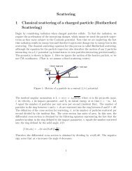
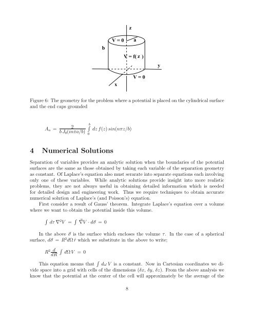
Figure 6: The geometry for the problem where a potential is placed on the cylindrical surface
and the end caps grounded
A n =
2
bJ 0 (inπa/b)
∫ b
0
dz f(z) sin(nπz/b)
4 Numerical Solutions
Separation of variables provides an analytic solution when the boundaries of the potential
surfaces are the same as those obtained by taking each variable of the separation geometry
as constant. Of Laplace’s equation also must serarate into separate equations each involving
only one of these variables. While analytic solutions provide insight into more realistic
problems, they are not always useful in obtaining detailed information which is needed
for detailed design and engineering work. Thus we require techniques to obtain accurate
numerical solution of Laplace’s (and Poisson’s) equation.
First consider a result of Gauss’ theorem. Integrate Laplace’s equation over a volume
where we want to obtain the potential inside this volume.
∫
dτ ∇ 2 V = ∫ ⃗ ∇V · d⃗σ = 0
In the above ⃗σ is the surface which encloses the volume τ. In the case of a spherical
surface, d⃗σ = R 2 dΩ ˆr which we substitute in the above to write;
R 2 d
dR
∫
dΩV = 0
This equation means that ∫ dω V is a constant. Now in Cartesian coordinates we divide
space into a grid with cells of the dimensions (δx, δy, δz). From the above analysis we
know that the potential at the center of the cell will approximately be the average of the
8