Solution to Laplace's Equation in Cylindrical Coordinates 1 ...
Solution to Laplace's Equation in Cylindrical Coordinates 1 ...
Solution to Laplace's Equation in Cylindrical Coordinates 1 ...

Create successful ePaper yourself
Turn your PDF publications into a flip-book with our unique Google optimized e-Paper software.
<strong>Solution</strong> <strong>to</strong> Laplace’s <strong>Equation</strong> <strong>in</strong> Cyl<strong>in</strong>drical<br />
Coord<strong>in</strong>ates<br />
Lecture 8<br />
1 Introduction<br />
We have obta<strong>in</strong>ed general solutions for Laplace’s equation by separtaion of variables <strong>in</strong> Cartesian<br />
and spherical coord<strong>in</strong>ate systems. The last system we study is cyl<strong>in</strong>drical coord<strong>in</strong>ates,<br />
but remember Laplaces’s equation is also separable <strong>in</strong> a few (up <strong>to</strong> 22) other coord<strong>in</strong>ate<br />
systems. As you know, choose the system <strong>in</strong> which you can apply the appropriate boundry<br />
conditions. It is only through application of the boundry conditions (Dirichlet of Neumann<br />
on a closed surface) that one f<strong>in</strong>ds a unique solution <strong>to</strong> the problem studied. In cyl<strong>in</strong>drical<br />
coord<strong>in</strong>ates apply the divergence of the gradient on the potential <strong>to</strong> get Laplace’s equation.<br />
∇ 2 V (ρ, φ, z) = ρ ∂2 V<br />
∂ρ 2 + ∂V<br />
∂ρ + (1/ρ) ∂2 V<br />
∂φ 2 + ∂2 V<br />
∂z 2 = 0<br />
We look for a solution by separation of variables;<br />
V = R(ρ)Ψ(φ)Z(z)<br />
As previously, this yields 2 separation constants, k and ν, which will lead <strong>to</strong> 2 eigenfunction<br />
equations. The three separated ode equations are;<br />
d 2 Z<br />
dz 2 − k 2 Z = 0<br />
d 2 Ψ<br />
dφ 2 + νΨ = 0<br />
d 2 R<br />
dρ 2 + (1/ρ) R dρ + (k2 − (ν/ρ) 2 )R = 0<br />
The later 2 equations can be set up as eigenfunction equations. The solutions are;<br />
Z ∝ e ±kz<br />
Ψ ∝ e ±iνφ<br />
R ∝ J ν (kρ), or/andN ν (kρ)<br />
1
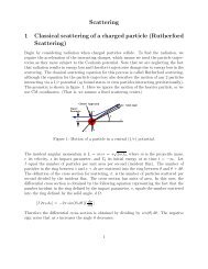
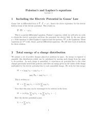
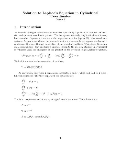
Figure 1: An example of the Cyl<strong>in</strong>drical Bessel function J(x) as a function of x show<strong>in</strong>g the<br />
oscillal<strong>to</strong>ry behavior<br />
2 Bessel Functions<br />
In the last section, J ν (kρ), N ν (kρ) are the 2 l<strong>in</strong>early <strong>in</strong>dependent solutions <strong>to</strong> Bessel’s equation.<br />
Bessel functions oscillate but not harmonically, see Figure 1. Thus we expect that<br />
the harmonic function solutions for Ψ and the Bessel function solutions for R will be the<br />
eigenfunctions when the boundry conditions are imposed. The Bessel functions, J ν (x), are<br />
regular at x = 0, while the Bessel functions, N ν (x), are s<strong>in</strong>gular at x = 0.<br />
The limit<strong>in</strong>g values of the Bessel functions are;<br />
lim x→0 J ν (x) → ( x 2 )ν<br />
[<br />
(2/π) ln(x) ν = 0<br />
]<br />
lim x→0 N ν (x) →<br />
(2/x) ν Γ(ν)<br />
π otherwise<br />
√<br />
lim x→∞ J ν (x) → 2 πx cos(x − νπ/2 − π/4)<br />
lim x→∞ N ν (x) →<br />
√<br />
2<br />
πx s<strong>in</strong>(x − νπ/2 − π/4)<br />
From the requirement that the solution be s<strong>in</strong>gle valued as φ → 2π, ie the solution is<br />
must not change when φ is replaced by φ+2π, the values of ν are <strong>in</strong>tegral and this produces<br />
eigenfuntions of Ψ. The series solution for the Bessel function J ν can be found by the method<br />
of Frobenius. However, the second l<strong>in</strong>early <strong>in</strong>dependent equation is not easily obta<strong>in</strong>ed when<br />
n is an <strong>in</strong>teger, and another technique is required. The Bessel function takes the form;<br />
2
J ν (x) = ∞ ∑<br />
s=0<br />
(−1) s<br />
s!(ν + s)! (x/2)ν+2s = xν<br />
2 n n! − x ν+2<br />
2 ν+2 (ν + 1)! + · · ·<br />
For <strong>in</strong>tegral values of ν one can show J −ν = (−1) ν J ν . The Bessel functions also satisfy the<br />
recurrence relations;<br />
J ν−1 (x) + J ν+1 (x) = ν x J ν(x)<br />
J ν−1 (x) = x ν J ν(x) + dJ ν<br />
dx<br />
d<br />
dx [xν J ν (x)] = x ν J ν−1<br />
At times an <strong>in</strong>tegral representation is useful.<br />
J ν (x) = (1/π)<br />
π∫<br />
0<br />
dθ e ix cos(θ) cos(νθ)<br />
The Bessel functions are orthogonal;<br />
∞∫<br />
0<br />
∫ a<br />
0<br />
kdk J ν (kρ) J ν (kρ ′ ) = δ(r − r ′ )/r<br />
ρdρ J ν (α νk ρ/a) J ν (α ′ νk ρ/a) = (a2 /2)[J ν+1 (α νk )] 2 δ kk ′<br />
In the above α νk are the zeros of the Bessel function of order ν where k orders these zeros.<br />
As the Bessel functions form a complete set, any function may be expanded <strong>in</strong> a Bessel series<br />
or <strong>in</strong>tegral for an <strong>in</strong>f<strong>in</strong>ite space.<br />
F(ρ) = ∫ kdk A(k) J ν (kρ)<br />
3 Examples<br />
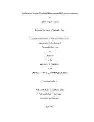
We f<strong>in</strong>d the solution for the <strong>in</strong>terior of a cyl<strong>in</strong>drical shell with the <strong>to</strong>p end cap held at a<br />
potential V = V 0 (ρ) and all the other surfaces grounded, Figure 2. The solution we seek<br />
has the form;<br />
V = ∑ νn<br />
A νkn J ν (k n ρ)s<strong>in</strong>h(k n z)e iνφ<br />
In this case the solution is <strong>in</strong>dependent of the angle φ so we take ν = 0. Note that we have<br />
not <strong>in</strong>cluded N ν <strong>in</strong> the solution because we want it <strong>to</strong> be f<strong>in</strong>ite as ρ = 0. Also we have chosen<br />
s<strong>in</strong>h(k n z) <strong>to</strong> satisfy the boundary condition at z = 0. The reduced solution is;<br />
3
L<br />
z<br />
V = Vo<br />
V = 0<br />
x<br />
V = 0<br />
a<br />
y<br />
Figure 2: The geometry of a cyl<strong>in</strong>der with one eddcap held at potential V = V 0 (ρ) and the<br />
other sides grounded<br />
V = ∑ n<br />
A n J 0 (k n ρ)s<strong>in</strong>h(k n z)<br />
Now V = 0 for ρ = a. This means that;<br />
J 0 (k n a) = 0<br />
The values of k n a are the zeros of the bessel function J 0 (k n a). The first few are, α 0n =<br />
2.4048, 5.5201, 8.6537, · · ·. Then at Z = L we f<strong>in</strong>d A n us<strong>in</strong>g the orthogonality of the Bessel<br />
functions.<br />
A n = 1<br />
a 2 [J 1 (k n a)] 2 s<strong>in</strong>h(k n L)<br />
∫ a<br />
0<br />
ρdρ J 0 (k n ρ) V 0 (ρ)<br />
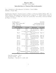
The graphic form of the solution is shown <strong>in</strong> figure 3.<br />
As another example we f<strong>in</strong>d the potential <strong>in</strong>side a cyl<strong>in</strong>der when the potential is specified<br />
on the end caps and the cyl<strong>in</strong>drical wall is at zero potential, figure 4. The boundry<br />
conditions are that;<br />
V = V 0 s<strong>in</strong>(φ)<br />
z = L<br />
V = −V 0 s<strong>in</strong>(φ) z = -L<br />
V = 0<br />
ρ = a<br />
The solution must have the form;<br />
4
Figure 3: A graphical representation of the above solution<br />
V = Vo s<strong>in</strong>( φ )<br />
z<br />
a<br />
L<br />
y<br />
x<br />
V = 0<br />
−L<br />
V = −Vo s<strong>in</strong>( φ )<br />
Figure 4: The geometry of the problem with endcaps held at potential V = V 0 ± s<strong>in</strong>(φ)<br />
5
z<br />
b<br />
c<br />
a<br />
V = f( ρ )<br />
V = 0<br />
y<br />
x<br />
Figure 5: The geometry for the problem of two concentric cyl<strong>in</strong>ders<br />
V = ∑ νn<br />
A νn J ν (k n ρ) s<strong>in</strong>(νφ) s<strong>in</strong>h(k n z)<br />
Here we have discarded solutions <strong>in</strong> N νn (kρ) which are <strong>in</strong>f<strong>in</strong>ite at the orig<strong>in</strong>. To match the<br />
boundry at z = ±L we need <strong>to</strong> have a term s<strong>in</strong>(νφ) which requires ν = 1. Then we require<br />
that the Bessel function, J 1n (k n a) = 0 which determ<strong>in</strong>es the zeros of the Bessel function of<br />
order 1. We write these as α 1n so that k n = α 1n /a. The solution then has the form;<br />
V = ∑ n<br />
A n J 1 (α 1n ρ/a) s<strong>in</strong>h(αz/a) s<strong>in</strong>(φ)<br />
F<strong>in</strong>ally we match the boundry condition at z = ±L where V = V 0 s<strong>in</strong>(φ). Use orthorgonality<br />
<strong>to</strong> obta<strong>in</strong>;<br />
(L/2)[J 1 (α 1n )] 2 A n = 1<br />
s<strong>in</strong>h(αL/a)<br />
∫ a<br />
0<br />
ρdρ J 1 (α 1n ρ/a) V 0<br />
As another example we look at a solution for concentric cyl<strong>in</strong>ders with the boundry<br />
conditions;<br />
r = a, c and z = 0 V = 0<br />
z = b V = f(ρ)<br />
This geometry is shown <strong>in</strong> Figure 5. We choose a solution <strong>to</strong> have the form;<br />
∑<br />
V = ∞ A n s<strong>in</strong>h(k n z) G 0 (k n ρ)<br />
n<br />
Here we have written a superposition of the Bessel and Neumann functions;<br />
6
G 0 = [ J 0(k n ρ)<br />
J 0 (k n c) − N 0(k n ρ)<br />
N 0 (k n c) ]<br />
So that at ρ = c, the cyl<strong>in</strong>drical surface of the <strong>in</strong>ner cyl<strong>in</strong>der, G 0 vanishes. Note we have<br />
chosen ν = 0 because the potential is <strong>in</strong>dependent of φ, ie the problem is aximuthally symmetric.<br />
Now we must choose the values of k n <strong>to</strong> make G 0 = 0 when ρ = a. This will select<br />
a set of zeros, α νn , of the function, G 0 , and <strong>in</strong> fact make the functions, G 0 , a complete<br />
orthogonal set. This po<strong>in</strong>ts out that we separated the solutions of the radial ode <strong>in</strong><strong>to</strong> a<br />
form which was regular at ρ = 0 and one which was not. But we could have separated the<br />
solutions so that, G 0 , was one of the two l<strong>in</strong>early <strong>in</strong>dependent solutions, and thus it would<br />
have similar oscillat<strong>in</strong>g properties as the function J ν . Of course the location of the zeros<br />
would be different. Use orthogonality <strong>to</strong> obta<strong>in</strong> the coefficients <strong>in</strong> the above equation.<br />
Here;<br />
H A n = [1/s<strong>in</strong>h(k n b)]<br />
H =<br />
∫ a<br />
c<br />
ρdρ G 2 (α n ρ/a)<br />
∫ a<br />
c<br />
ρdρ V (ρ) G(α n ρ/a)<br />
F<strong>in</strong>ally consider the problem with the cyl<strong>in</strong>drical wall held at potential V = f(z) and<br />
the endcaps grounded. This geometry is shown <strong>in</strong> figure 6. The boundry conditions are;<br />
z = 0, b V = 0<br />
ρ = a V = f(z)<br />
In this case we cannot use the hyperbolic function <strong>in</strong> z <strong>to</strong> match the boundry conditions.<br />
However if we let k → ik then the hyperbolic function becomes harmonic at the expense of<br />
mak<strong>in</strong>g the argument of the Bessel function complex. Note here that the problem is 2-D<br />
so we expect only one eigenfunction and this now occurs for the z coord<strong>in</strong>ate. Then the<br />
radial ode with complex Bessel function solutions cannot be eigenfunctions. The eigenvalue<br />
of k = nπ/b is determ<strong>in</strong>ed by the harmonic form;<br />
s<strong>in</strong>(nπz/b)<br />
n <strong>in</strong>tegral<br />
The solution has the form;<br />
V = ∞ ∑<br />
n=1<br />
A n s<strong>in</strong>(nπz/b) J 0 (<strong>in</strong>πρ/b)<br />
In this case we use the orthogonality of the harmonic functions rather than the Bessel functions.<br />
The value of the coefficients are;<br />
7
V = 0<br />
z<br />
a<br />
z V = f( )<br />
y<br />
x<br />
V = 0<br />
Figure 6: The geometry for the problem where a potential is placed on the cyl<strong>in</strong>drical surface<br />
and the end caps grounded<br />
A n =<br />
2<br />
bJ 0 (<strong>in</strong>πa/b)<br />
∫ b<br />
0<br />
dz f(z) s<strong>in</strong>(nπz/b)<br />
4 Numerical <strong>Solution</strong>s<br />
Separation of variables provides an analytic solution when the boundaries of the potential<br />
surfaces are the same as those obta<strong>in</strong>ed by tak<strong>in</strong>g each variable of the separation geometry<br />
as constant. Of Laplace’s equation also must serarate <strong>in</strong><strong>to</strong> separate equations each <strong>in</strong>volv<strong>in</strong>g<br />
only one of these variables. While analytic solutions provide <strong>in</strong>sight <strong>in</strong><strong>to</strong> more realistic<br />
problems, they are not always useful <strong>in</strong> obta<strong>in</strong><strong>in</strong>g detailed <strong>in</strong>formation which is needed<br />
for detailed design and eng<strong>in</strong>eer<strong>in</strong>g work. Thus we require techniques <strong>to</strong> obta<strong>in</strong> accurate<br />
numerical solution of Laplace’s (and Poisson’s) equation.<br />
First consider a result of Gauss’ theorem. Integrate Laplace’s equation over a volume<br />
where we want <strong>to</strong> obta<strong>in</strong> the potential <strong>in</strong>side this volume.<br />
∫<br />
dτ ∇ 2 V = ∫ ⃗ ∇V · d⃗σ = 0<br />
In the above ⃗σ is the surface which encloses the volume τ. In the case of a spherical<br />
surface, d⃗σ = R 2 dΩ ˆr which we substitute <strong>in</strong> the above <strong>to</strong> write;<br />
R 2 d<br />
dR<br />
∫<br />
dΩV = 0<br />
This equation means that ∫ dω V is a constant. Now <strong>in</strong> Cartesian coord<strong>in</strong>ates we divide<br />
space <strong>in</strong><strong>to</strong> a grid with cells of the dimensions (δx, δy, δz). From the above analysis we<br />
know that the potential at the center of the cell will approximately be the average of the<br />
8
potential over the enclos<strong>in</strong>g surface. In Cartesian coord<strong>in</strong>ates this means that the potential<br />
at a po<strong>in</strong>t is approximately the average of the sum of the potentials over its nearest neighbors.<br />
V l,m,n = 1/6[V l−1,m,n + V l+1,m,n + V l,m−1,n +<br />
V l,m+1,n + V l,m−1,n + V l,m,n−1 + V l,m,n+1 ]<br />
One beg<strong>in</strong>s by tak<strong>in</strong>g the exact potential values on the surface and assign<strong>in</strong>g <strong>in</strong>itial<br />
values <strong>to</strong> the potential at all the grid po<strong>in</strong>ts. The <strong>in</strong>itial values can be any guesses. The<br />
average values at each po<strong>in</strong>t are then obta<strong>in</strong>ed, keep<strong>in</strong>g the correct potential on the surface.<br />
The process is iterated <strong>to</strong> convergence. The thechnique is called the relaxation method. It<br />
is stable by iteration and converges rapidly <strong>to</strong> the potential with<strong>in</strong> a volume. This technique<br />
(f<strong>in</strong>ite element analysis) is generally applied <strong>to</strong> any process which is described by Laplace’s<br />
equation, and this <strong>in</strong>cludes a number of physical processes <strong>in</strong> addition <strong>to</strong> electrostatics.<br />
If charge is present, we must have a solution <strong>to</strong> Poisson’s equation. For a sphere of<br />
radius, r, the potential at the center relative <strong>to</strong> the surface is;<br />
∆V = ρr 2 /(6ǫ 0 )<br />
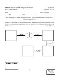
This would be <strong>in</strong>cluded <strong>in</strong> the equation above when comput<strong>in</strong>g the average. As an example,<br />
Figure 7 shows a numerical valuation of a potential at the center of a set of grounded<br />
metal boundaries and wires which are held at constant potential.<br />
9
Figure 7: An 3-D numerical example show<strong>in</strong>g con<strong>to</strong>ur l<strong>in</strong>es of constant potential of a geometry<br />
hav<strong>in</strong>g grounded metal boundaries and wires held at potential<br />
10