
You also want an ePaper? Increase the reach of your titles
YUMPU automatically turns print PDFs into web optimized ePapers that Google loves.
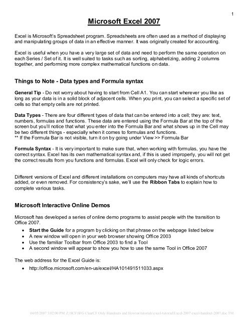
<strong>Microsoft</strong> <strong>Excel</strong> 2007<br />
<strong>Excel</strong> is <strong>Microsoft</strong>’s Spreadsheet program. Spreadsheets are often used as a method of displaying<br />
and manipulating groups of data in an effective manner. It was originally created for accounting.<br />
<strong>Excel</strong> is useful when you have a very large set of data and need to perform the same operation on<br />
each Series / Set of it. It is well suited to tasks such as sorting, alphabetizing, adding 2 columns<br />
together, and performing more complex mathematical functions on data.<br />
Things to Note - Data types and Formula syntax<br />
General Tip - Do not worry about having to start from Cell A1. You can start wherever you like as<br />
long as your data is in a solid block of adjacent cells. When you print, you can select a specific set of<br />
cells so that empty cells are not printed.<br />
Data Types - There are four different types of data that can be entered into a cell; they are: text,<br />
numbers, formulas and functions. These data are entered using the Formula Bar at the top of the<br />
screen but you’ll notice that what you enter into the Formula Bar and what shows up in the Cell may<br />
be two different things - especially when it comes to formulas and functions.<br />
** If the Formula Bar is not visible, turn it on by going under View >> Formula Bar<br />
Formula Syntax - It is very important to make sure that, when working with formulas, you have the<br />
correct syntax. <strong>Excel</strong> has its own mathematical syntax and, if this is used improperly, you will not get<br />
the correct results from you functions and formulas. <strong>Excel</strong> will only check for logic errors.<br />
Different versions of <strong>Excel</strong> and different installations on computers may have all kinds of shortcuts<br />
added, or even removed. For consistency’s sake, we’ll use the Ribbon Tabs to explain how to<br />
complete various tasks.<br />
<strong>Microsoft</strong> Interactive Online Demos<br />
<strong>Microsoft</strong> has developed a series of online demo programs to assist people with the transition to<br />
Office 2007.<br />
� Start the Guide for a program by clicking on that phrase on the webpage listed below<br />
� A new window will open in your web browser showing Office 2003<br />
� Use the familiar Toolbar from Office 2003 to find a Tool<br />
� A second window will appear to show you how to use the same Tool in Office 2007<br />
The web address for the <strong>Excel</strong> Guide is:<br />
� http://office.microsoft.com/en-us/excel/HA101491511033.aspx<br />
04/05/2007 3:02:00 PM Z:\SCF\SFG ClearCF Only\Handouts and Howtos\tutorials\excel-tutorial\<strong>Excel</strong>-2007\excel-handout-2007.doc TM<br />
1
MS EXCEL 2007 - New Interface<br />
When you open <strong>Excel</strong> 2007, you will notice that it looks quite different from <strong>Excel</strong> <strong>2000</strong> and <strong>Excel</strong> 2003. The<br />
same tools are all there, but they are arranged very differently and new features have been added.<br />
If you are already familiar with <strong>Excel</strong> <strong>2000</strong> or 2003, it may take you a while to adjust to this new arrangement of<br />
tools. This tutorial uses <strong>Excel</strong> 2007 and you can use it as a quick reference guide for most of the common<br />
tools.<br />
Arrangement of Tools in <strong>Excel</strong> 2007<br />
The MS Office Button contains the main file functions<br />
� New, Open, Save, Save as, Print, Print Preview, etc.<br />
The Quick Access Toolbar contains shortcuts to Save, Undo, and Repeat<br />
Each Ribbon Tab displays a Ribbon that provides a set of<br />
Tool Groups.<br />
� The Ribbon Tab and the Tool Groups in the Ribbon<br />
correspond to the Menu and Toolbar in Word <strong>2000</strong> and<br />
2003<br />
� The Name of each Tool Group is listed at the bottom of<br />
the Group<br />
o Example - In the Home Tab, the second Tool<br />
Group is named Font<br />
o The name "Font" is under the Font Tool Group<br />
To change the Tool Groups being displayed in the Ribbon<br />
� Click on the appropriate Ribbon Tab<br />
� Example - The Home Tab contains Tool Groups for the most commonly used Tools<br />
o ClipBoard, Font, Paragraph, and Style tools in Word<br />
Some Tool Group boxes have a small arrow in the bottom right-hand corner.<br />
� If you click on this arrow, Word will open a Dialog Box which offers<br />
more options and settings related to that Tool Group<br />
In <strong>Excel</strong> 2007, tools with similar uses are organized so that they are usually found within the same Tool Group<br />
or at least within one Ribbon. If you do not find a tool in the Ribbon you think it should be in, try exploring the<br />
other Ribbon Tabs.<br />
In this tutorial, we will not use the control keys as these function differently on different computers. For the sake<br />
of consistency, all instructions in this tutorial refer to the Ribbon Tabs and Tool Groups in each Ribbon.<br />
04/05/2007 3:02:00 PM Z:\SCF\SFG ClearCF Only\Handouts and Howtos\tutorials\excel-tutorial\<strong>Excel</strong>-2007\excel-handout-2007.doc TM<br />
2
Start a new Workbook MS Office Button >> New<br />
Open an existing<br />
Workbook<br />
Open a file from a<br />
different version or<br />
format<br />
Getting Started<br />
When you open <strong>Excel</strong> for the first time, a new, blank Workbook appears.<br />
If you are already in <strong>Excel</strong> and want a new Workbook<br />
� Click on MS Office Button and choose New<br />
NOTE: In <strong>Excel</strong>, a Workbook is the basic document<br />
� Each Workbook contains several Sheets on which different sets of Data can be<br />
entered<br />
� The Sheets are listed at the bottom of the <strong>Excel</strong> window<br />
� Sheets can be given individual names<br />
� Click on the name of a each sheet to switch between them<br />
MS Office Button >> Open<br />
� Browse to an <strong>Excel</strong> Workbook document and Open it<br />
<strong>Excel</strong> 2007 will automatically convert a document from a compatible version of <strong>Excel</strong><br />
� Your document will open in Compatibility Mode<br />
� This will prevent you from using certain tools in Office 2007 which are not<br />
compatible with Office <strong>2000</strong> or 2003<br />
� When you finish editing a document, be VERY CAREFUL to save any converted<br />
documents in their original format<br />
� Please read the Important Notes below regarding saving in Office 2007!<br />
IMPORTANT NOTES: Saving Documents in <strong>Excel</strong> 2007<br />
1. In the Computing Facilities, files on the Desktop are NOT SAVED when you log off.<br />
� ALWAYS use Save As... to save your file to a USB Flash Drive, UVicTemp, or CD<br />
� You can also save a file to the Desktop and then email it to yourself as an attachment<br />
2. If you are NOT running Office 2007 at home and you save a document as <strong>Excel</strong> 2007 (*.xlsx),<br />
YOU WILL NOT BE ABLE TO OPEN IT AT HOME! (see step 3 below)<br />
3. If you have Office <strong>2000</strong> or 2003 or you use a Mac at home or in the Computing Facilities<br />
� You will have to save your document as an older version<br />
� Go to MS Office Button >> Save As<br />
o At the bottom, there is a bar that asks you to “Save as Type:”<br />
o Choose <strong>Excel</strong> 97-2003 Workbook (*.xls)<br />
� DO NOT CHOOSE “<strong>Excel</strong> Workbook (*.xlsx)”<br />
4. If you are using a PC at home running Office <strong>2000</strong> or 2003<br />
� You can download the MS Office 2007 to Office 2003 Compatibility Pack from <strong>Microsoft</strong>'s website<br />
o http://www.microsoft.com/downloads/<br />
o Under New Downloads, choose "<strong>Microsoft</strong> Office Compatibility Pack for Word..."<br />
� Even with the Compatibility Pack, you might lose data / formatting when you save as an older version<br />
� There is no Compatibility Pack available for Mac yet.<br />
Save the current<br />
Workbook<br />
OR<br />
Save the Workbook<br />
as a different name,<br />
version, or format<br />
MS Office Button >> Save or Save As...<br />
� Please read the Important Notes above regarding saving in Office<br />
2007!<br />
� In the bars at the bottom of the Save As... Window<br />
� Give your document a new name in “File Name:”<br />
� Select the version and format from “Save as type:”<br />
04/05/2007 3:02:00 PM Z:\SCF\SFG ClearCF Only\Handouts and Howtos\tutorials\excel-tutorial\<strong>Excel</strong>-2007\excel-handout-2007.doc TM<br />
3
Formatting Data<br />
Insert Data into a cell Select a Cell by placing the cursor in the Cell<br />
Insert more Cells into<br />
a Sheet<br />
Change the Type of<br />
Data within a Cell<br />
or cells<br />
(Ex: increase decimal<br />
places)<br />
Change the Font of<br />
the Data in a Cell<br />
Change the Alignment<br />
of the Data in a Cell<br />
� Type data into the Formula Bar at the top of the <strong>Excel</strong> Window<br />
� OR into the Cell directly<br />
� Data can be - Number, Text, Formula, or Function<br />
Home Tab - Font, Alignment, Number & Cell Groups<br />
Home Tab >> Cells Group<br />
� Place the cursor where you want the Cells to be added or deleted<br />
� Choose the Insert or Delete Tool in the Cells Group<br />
� You can add Cells, Rows, Columns, or a whole new Sheet for Data<br />
Home Tab >> Number Group<br />
Select the cell(s) you wish to format<br />
� Click on the pull-down menu at the top of the Number Group<br />
o If you move the mouse over this menu, it says Number Format<br />
� Assign a Data Type to the Cell(s)<br />
� "General" is the Default Data Type<br />
Home Tab >> Font Group<br />
� Select the cell(s) you wish to format<br />
� In the Font Group there are several Tools for altering the Font, Size, Colour, and<br />
Style of the Data in the Cell<br />
Home Tab >> Alignment Group<br />
� Select the cell(s) you wish to format<br />
� In the Alignment Group there are Tools for<br />
o Centring Data in Cells Horizontally and Vertically<br />
o Merging and Un-Merging Cells<br />
o Wrapping Data so that it continues to the next line within one Cell<br />
04/05/2007 3:02:00 PM Z:\SCF\SFG ClearCF Only\Handouts and Howtos\tutorials\excel-tutorial\<strong>Excel</strong>-2007\excel-handout-2007.doc TM<br />
4
Format Cells Dialog Box - (has not changed from Word <strong>2000</strong>, 2003)<br />
� Allows you to change several properties of a Cell within one Dialog<br />
Box.<br />
o Type of Data<br />
o Alignment/Position of Data in a Cell<br />
o Font of the Data<br />
o Cell Borders and Fill<br />
� Offers more options than the Tool Groups in the Ribbon<br />
� It is especially useful for altering Cell Borders<br />
� To Open or Launch the Format Cells Box<br />
o Select the cells you wish to format<br />
o Click on the Dialog Box Launcher arrow at the right bottom corner of the<br />
Font, Alignment, or Number Groups<br />
Format the<br />
Borders of Cells<br />
Format the Column<br />
Width or Row<br />
Height of Cells<br />
Home Tab >> Launch Format Dialog Box<br />
(small arrow at bottom right of Groups)<br />
Select the Cell(s) you wish to format<br />
� Click on the Dialog Box Launcher arrow at<br />
the right bottom corner of the<br />
� Font, Alignment, or Number Groups<br />
� This will launch the Format Cells Dialog Box<br />
� Click on the Border Tab at the top of this Box<br />
1. Choose a Style of Line<br />
2. Choose a Colour for the Line<br />
3. Choose which Border Lines you want to<br />
see around the Cell(s)<br />
Home Tab >> Cells Group >> Format<br />
Select the Cell(s) for which you want to change the Row Height or<br />
Column Width<br />
� Click on the Format button in the Cells Group<br />
� Choose to adjust the Column Width or Row Height<br />
OR<br />
� Select Autofit to adjust the Cell to the size of the Data<br />
Move a cell(s) � Select the Cell(s) you want to move<br />
� Position the mouse over a border of the selection<br />
� The cursor will change from a thick white plus sign into thin crossed arrows<br />
� Click-drag the cells to their destination.<br />
Merge Cells<br />
Combine several<br />
Cells into 1<br />
NOTE:<br />
This process ONLY<br />
retains Data from<br />
the top left Cell<br />
Home Tab >> Alignment Group >> Merge & Center<br />
Select the Cell(s) to be Merged<br />
� Click on the Merge & Center Tool<br />
� Select Merge Cells from the pull-down<br />
menu<br />
OR<br />
� Launch the Format Dialog Box using<br />
the arrow at the bottom right corner of the Alignment Group<br />
� Check the Merge Cells box under Text Control.<br />
04/05/2007 3:02:00 PM Z:\SCF\SFG ClearCF Only\Handouts and Howtos\tutorials\excel-tutorial\<strong>Excel</strong>-2007\excel-handout-2007.doc TM<br />
5
Automatically fill<br />
Data Cells<br />
<strong>Excel</strong> can automatically continue a list if you provide the first 2 or 3 items in it. This is<br />
very useful for basic sequences such as:<br />
� Days of the week<br />
� List of numbers<br />
Input data into a Cell or across two consecutive cells to get an incremental list<br />
� Select the cell(s)<br />
� Position the mouse in bottom right corner of the selection<br />
� The pointer will change to a thin black cross<br />
� Click-drag downwards or to the right across the neighbouring empty cells to<br />
apply the Auto-fill to all desired cells<br />
Sorting Data Data Tab >> Sort & Filter Group >> Sort<br />
Select the Data in a Row or Column<br />
� Click on the Sort button to open the Sort<br />
window<br />
Home Tab >> Editing >> Sort & Filter<br />
For simple Sorting, use the Sort & Filter Tool in<br />
the Editing Group of the Home Tab<br />
Formulas are entered in the Formula Bar under the<br />
Ribbon.<br />
Formulas are composed of one or more Functions.<br />
Formulas - The Formula Bar & Functions<br />
Formulas:<br />
� Require an equals sign to begin '='<br />
� Follow the rules of BEDMAS (see below)<br />
� Will be checked for Notation errors, not Logic errors<br />
� Rely on column/row numbering (A1, Z39)<br />
� Are most easily tackled by using the online help feature<br />
To begin a Formula:<br />
Select the Cell where you want the result to<br />
appear<br />
� This Cell does not have to be adjacent to<br />
the Data used by the Formula<br />
1. Type an equals sign '=' into either<br />
o The Formula Bar<br />
o The Cell where you want the Result to<br />
appear<br />
2. Choose a Function from the Function List<br />
to the left of the Formula Bar<br />
o This list contains commonly used<br />
Functions such as Add or Sum<br />
o For more functions, choose More<br />
Functions...<br />
o The Insert Function Dialog Box will<br />
open<br />
3. The Result of the Function will appear in the<br />
Cell you chose in Step 1<br />
04/05/2007 3:02:00 PM Z:\SCF\SFG ClearCF Only\Handouts and Howtos\tutorials\excel-tutorial\<strong>Excel</strong>-2007\excel-handout-2007.doc TM<br />
6
Functions &<br />
Operators for<br />
Formulas<br />
AutoSum<br />
Automatically Sum<br />
your Data<br />
Inserting a Chart<br />
from Data<br />
Operations follow the order of BEDMAS:<br />
� Brackets, Exponents, Divide, Multiply, Add, Subtract<br />
Formula Notation for common mathematical functions<br />
Addition: +<br />
Subtraction: -<br />
Division: \<br />
Multiplication: *<br />
Brackets: ( )<br />
Range: ... [i.e. A1...A70]<br />
Home Tab >> Editing Group >> AutoSum<br />
<strong>Excel</strong> can automatically, quickly, Add a row or column of<br />
numbers for you:<br />
� Select the Cells you want to sum<br />
� Include an empty Cell as the last Cell in the selection<br />
� This is where your summation result will be entered<br />
� Click on the AutoSum Tool in the Editing Group<br />
� Choose Sum from the list<br />
Several other commonly used Functions are available here such as:<br />
� Average, Count, Min, Max<br />
To automatically apply the same Function to a Set of Cells<br />
� Follow instructions to Automatically Fill Data Cells on page 6 above<br />
Creating and Formatting Charts<br />
Insert Tab >> Charts Group<br />
� Select a set of Data<br />
o The Data should all be adjacent and arranged in Columns<br />
o The leftmost Column is Data for the X-Axis<br />
o Each other Column represents a different Series of Data or Set of Y-Values<br />
� Choose a Chart Type (Column, Pie, Scatter, etc.) from the Charts Group<br />
� Or click on Dialog Box Launcher arrow at the right bottom corner of Chart Group<br />
to launch Insert Chart window<br />
� Select the type of chart you want<br />
Choose the type of Chart you want.<br />
� XY (Scatter) is one of the more popular Chart Types for representing data because<br />
it allows you to alter both the X-axis and the Y-axis<br />
� There are several other types of charts and each has different options for laying out<br />
data. See which one works best for your data set<br />
NOTE :<br />
<strong>Excel</strong> 2007 has removed the Chart Wizard. You must use the<br />
Chart Tools Ribbon Tabs to format and alter the appearance and Data of your Chart.<br />
See instructions below.<br />
04/05/2007 3:02:00 PM Z:\SCF\SFG ClearCF Only\Handouts and Howtos\tutorials\excel-tutorial\<strong>Excel</strong>-2007\excel-handout-2007.doc TM<br />
7
Chart Tools Tab:<br />
� Design Tab<br />
� Layout Tab<br />
� Format Tab<br />
You need to use<br />
Chart Tools Tabs<br />
to Format any part<br />
of the Chart<br />
Creating a Chart<br />
Step 1<br />
Choose / Change a<br />
Chart Design<br />
Creating a Chart<br />
Step 2<br />
� Choose a Data<br />
Range<br />
� Add or Delete a<br />
Series<br />
Series - a single<br />
Column of Data<br />
1. To Format a Chart, always Select the Chart first by clicking on it.<br />
2. Chart Tools Tab appears providing the Design Tab, Layout Tab and Format Tab<br />
for Formatting the selected Chart<br />
Chart Tools - Design Tab >> Type Group >> Change Chart Type<br />
� Click on Change Chart Type Tool to change the type of chart<br />
Choose the type of Chart you want.<br />
� XY (Scatter) is one of the more popular Chart Types for representing data because<br />
it allows you to alter both the X-axis and the Y-axis<br />
� There are several other types of charts and each has different options for laying out<br />
data. See which one works best for your data set<br />
Formatting a Chart - Step 2 - Changing the Data Range for a Series<br />
Chart Tools - Design Tab >> Data Group >> Select Data<br />
NOTE: You only need to use the Select Data Tool if the Chart is NOT displaying the<br />
correct Data for each Series.<br />
� Click on Select Data button to change the Data Range of each Series of the Chart<br />
� The Select Data Source window will appear<br />
� Select a Data Series in the box on the left (Ex. "Jim")<br />
� Click on Edit button to change the Data in the Series<br />
o The Edit Series window will appear<br />
o To choose Data straight off the <strong>Excel</strong> Sheet, click on the Graph Symbol next<br />
to the Series Name, X-Values, or Y-Values<br />
� Click Delete in the Data Source window to Delete a Data Series<br />
04/05/2007 3:02:00 PM Z:\SCF\SFG ClearCF Only\Handouts and Howtos\tutorials\excel-tutorial\<strong>Excel</strong>-2007\excel-handout-2007.doc TM<br />
8
Creating a Chart<br />
Step 3<br />
Edit Chart Titles,<br />
Labels, Axis and<br />
Background<br />
Creating a Chart<br />
Step 4<br />
Chart Location<br />
Stretching the<br />
Chart<br />
Chart Tools - Layout Tab >> Labels, Axes, & Background Groups<br />
Labels Group:<br />
� Chart Title / Axis Titles Tools<br />
o Add, remove and position the titles of the chart and axis<br />
o To change the Font for a Title, highlight the text and go to the<br />
Font Group in the Home Tab<br />
� Legend Tool<br />
o Add, remove and position the Chart Legend<br />
o The Legend assigns a separate colour to each Data Series<br />
� Data Labels Tool<br />
o Data Labels are the X or Y values for each Data Point in a Series<br />
o They will appear next to each Data Point Marker in a Series Line<br />
o Add, remove and position the Data Labels<br />
� Data Table Tool<br />
o Add the Data Table to the chart<br />
Axes Group:<br />
� Axes Tool - Change the formatting and layout of each axis<br />
� Gridlines Tool - Turn Major and Minor Gridlines on or off<br />
Background Group: Edit the Background color and style of the chart.<br />
There are more options for all of these Groups.<br />
� Choose "More options" when you click on a Tool<br />
� A Format Dialog Box will open for that Tool<br />
� As you select each option, the Chart Preview will change. If you are unsure of what<br />
an option will do to your Chart, try clicking on it. You can always turn it off again.<br />
Chart Tools - Design Tab >> Location Group >> Move Chart<br />
� This Tool is located on the far right of the Chart Tools Design Tab<br />
� Choose whether you want the Chart to appear as an object on the same sheet as<br />
your data (more common) or on its own sheet<br />
If the Axis Labels are positioned too close together, or the Chart is not the shape you<br />
want it to be, you can stretch the chart.<br />
� Click in the blank background of the Chart near the Title. You should see a box<br />
appear around the entire Chart.<br />
� Click and drag the “handles” of the box to make the Chart bigger<br />
04/05/2007 3:02:00 PM Z:\SCF\SFG ClearCF Only\Handouts and Howtos\tutorials\excel-tutorial\<strong>Excel</strong>-2007\excel-handout-2007.doc TM<br />
9
Formatting Parts of a Chart<br />
There are two methods you can use to Format any part of your Chart<br />
Format the<br />
� Font, Colour, Shape, Fill, Outline or Style<br />
of the<br />
� Chart Area (background of whole chart), X or Y Axes, Legend,<br />
Plot Area, Gridlines, Titles, Data Series Lines, or Plot Points<br />
Method 1<br />
� Right-click on that specific part of the Chart and choose Format ____ ...<br />
Method 2<br />
Chart Tools - Format Tab >> Current Selection Group<br />
1. Click on the Chart Elements List.<br />
o A pull-down menu will list all the elements of your Chart<br />
o Select the part of the chart that you want to format<br />
2. Click on the Format Selection button<br />
o A Format Dialog Box will appear for that element of the chart<br />
Some parts in the chart (i.e. Lines and Plot Points) are easier to select by Method 2 than by right-clicking.<br />
Note: In the sections below, we mainly use the Right-click Method to select an area of the chart.<br />
Formatting Axes<br />
Change the Pattern,<br />
Scale, Font, Number<br />
Type, and Angle of<br />
the X and Y Axes.<br />
Of these, the most<br />
important is the<br />
Scale of the Axes.<br />
Right-click on the X or Y axis in your Chart and choose Format Axis...<br />
� The Format Axis Dialog Box will open<br />
Set the Axis options:<br />
� Axis Options - These greatly affect how your data is displayed!<br />
When the Chart is created, the major values (tick marks) of the axes are set<br />
automatically, but you might want them to be very different.<br />
Axis Options allows you to set:<br />
o Minimum and Maximum value for each axis<br />
o Major Unit - The increment between major values (tick marks) on the axis<br />
o Minor Unit - The increment between minor values (smaller tick marks) on the<br />
axis<br />
o To change any of these options, click on the Fixed, not Auto setting<br />
� Number - Change the Type of Data for the axis values (date, time, text...)<br />
� Fill, Line Colour, Line Style - Change the background color, Axis colour, or Axis<br />
Line style for the X or Y axis<br />
� Alignment - Change the direction of the text for the Axis Values<br />
04/05/2007 3:02:00 PM Z:\SCF\SFG ClearCF Only\Handouts and Howtos\tutorials\excel-tutorial\<strong>Excel</strong>-2007\excel-handout-2007.doc TM<br />
1<br />
Chart Elements List<br />
10
Formatting a<br />
Series of Data<br />
Change the<br />
appearance of a<br />
Data Series Line<br />
and its Markers<br />
Display and Format<br />
Data Labels<br />
Show the Data<br />
Values<br />
Data Labels<br />
The X or Y values<br />
can be displayed<br />
next to each Data<br />
Marker in a Series<br />
Line<br />
Adding Error Bars<br />
to a Series of Data<br />
Error Bar<br />
A small line<br />
extending from each<br />
Data Marker that<br />
represents the<br />
potential error of<br />
your data.<br />
Right-click on the Series Line and choose Format Data Series...<br />
� The Format Data Series Dialog Box will open<br />
Set the Data Series options:<br />
� Series Options - decide whether to place a series on a Primary or Secondary Axis<br />
� Marker Options and Fill - Change the Marker Shape, Colour, and Size<br />
� Marker Line Color & Style - Change the Color and Style of the Marker Outline<br />
� Line Color & Line Style - Change the Colour and Style of the Series Line<br />
Chart Tools - Layout Tab >> Labels Groups >> Data Labels<br />
To create Data Labels:<br />
� Select a Series Line<br />
� Click on the Data Labels Tool in the Labels Group<br />
� Choose a position for the Data Labels relative to<br />
their Marker<br />
To show the Format Data Labels Dialog Box:<br />
� Right-click on a Series Line that has Data Labels and choose<br />
Format Data Labels...<br />
� The Format Data Labels Dialog Box will open<br />
Set the Data Labels options:<br />
� Label Options - Choose which X or Y Value you want the Label to display and<br />
where you want the Label to be positioned relative to the Series Markers<br />
� Number - Change the Type of Data for the axis values (date, time, text...)<br />
� Fill, Border Colour, Border Style - Change the appearance of the Data Label<br />
� Alignment - Change the direction of the text in the Data Label<br />
Chart Tools - Layout Tab >> Analysis Group >> Error Bars<br />
To create Error Bars:<br />
� Select a Series Line<br />
� Click on the Error Bars Tool in the Analysis<br />
Group<br />
� Select the Type of Error Bars you want<br />
o Standard, Percentage, or Standard Deviation<br />
� Horizontal and Vertical Error Bars will appear<br />
on all the Data Markers in that Series Line<br />
� To Delete Horizontal or Vertical Error Bars, select<br />
one or the other and hit the Delete Key<br />
To show the Format Error Bars Dialog Box:<br />
� Select the Error Bars for a Series Line that has them<br />
� Right-click on an Error Bar and choose Format Error Bars...<br />
� The Format Error Bars Dialog Box will open<br />
Set the Error Bars options:<br />
� Vertical / Horizontal Error Bars<br />
o Show the Plus, Minus, or Both Error Bars<br />
o Amount of Error - Fixed, Percentage, Standard Deviation, Standard Error<br />
� Line Colour, Style - Change the appearance of the Error Bars<br />
04/05/2007 3:02:00 PM Z:\SCF\SFG ClearCF Only\Handouts and Howtos\tutorials\excel-tutorial\<strong>Excel</strong>-2007\excel-handout-2007.doc TM<br />
11
Creating Trend<br />
Lines and their<br />
Equations<br />
Trendline<br />
The line that best<br />
represents the<br />
average of your data<br />
points.<br />
<strong>Excel</strong> can provide<br />
an equation for the<br />
Trendline<br />
Set the Print Area<br />
of a spreadsheet<br />
Preview the<br />
print-out<br />
Chart Tools - Layout Tab >> Analysis Group >> Trendline<br />
To create a Trendline:<br />
� Select a Series Line<br />
� Click on the Trendline Tool in the Analysis<br />
Group<br />
� Select the type of Trendline you want<br />
o Linear, Exponential, Linear Forecast<br />
� A Trend Line will appear on your Chart and be<br />
added to the Legend<br />
To show the Format Trend Line Dialog Box:<br />
� Select a Trend Line and Right-click on it (or use the Chart Elements List)<br />
� Choose Format Trendline... and the Format Trendline Dialog Box will open<br />
Set the Trendline options:<br />
� Trendline Options<br />
o Type - Exponential, Linear, Logarithmic, Polynomial, Power,<br />
o Name - Change the Name of the Trendline in the Legend<br />
o Check Display Equation on Chart to show the Equation of the Trendline<br />
� This is one of the most useful features of <strong>Excel</strong>!<br />
� Line Color, Style - Change the appearance of the Trendline<br />
Printing<br />
Page Layout Tab >> Page Setup Group >> Print Area<br />
To print ONLY selected data<br />
� Select an area of Data in the Data Sheet<br />
you want to print<br />
� Click on the Print Area Tool in the Page<br />
Setup Group<br />
� Choose Set Print Area<br />
MS Office Button >> Print<br />
� Click on OK to print the Print Area<br />
MS Office Button >> Print<br />
� Place the mouse over Print to see more options<br />
� Choose Preview from the list in the right side of the MS Office Box<br />
NOTE: You may find that you need to set the Page Orientation to Landscape<br />
(Horizontal) to make your Data Sheet fit properly. Printing that spans several pages is<br />
available for larger spreadsheets.<br />
This tutorial covers the basic features of <strong>Excel</strong>. This handout can be used as a general reference tool. If you<br />
require further assistance, especially in creating Formulas, please ask Staff for assistance with any other<br />
aspect of <strong>Excel</strong>. Formula tutorials can also be found in <strong>Excel</strong>'s Help or online.<br />
Thank you for attending our <strong>Microsoft</strong> Office tutorial series.<br />
This tutorial series was originally developed by the E-Learning Systems Group (ESG)<br />
at UVic and has been expanded and re-written for use in the Student Computing Facilities.<br />
04/05/2007 3:02:00 PM Z:\SCF\SFG ClearCF Only\Handouts and Howtos\tutorials\excel-tutorial\<strong>Excel</strong>-2007\excel-handout-2007.doc TM<br />
12