Structure and evolution of an active region on the - prace

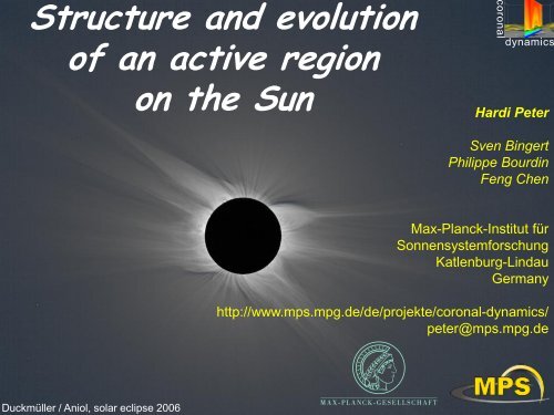
Duckmüller / Aniol, solar eclipse 2006
<strong>Structure</strong> <strong><strong>an</strong>d</strong> <strong>evolution</strong>
<strong>of</strong> <strong>an</strong> <strong>active</strong> <strong>region</strong>
oronal
dynamics
on the Sun
Hardi Peter
Sven Bingert
Philippe Bourdin
Feng Chen
Max-Pl<strong>an</strong>ck-Institut für
Sonnensystemforschung
Katlenburg-Lindau
Germ<strong>an</strong>y
http://www.mps.mpg.de/de/projekte/coronal-dynamics/
peter@mps.mpg.de

The corona <strong>of</strong> the Sun
> 1 000 000 K
visible
surface:
5800 K
How c<strong>an</strong> a cool body
heat its hot surroundings ?!
EUV / X-rays:
plasma at
> 10 6 K
solar eclipse 13.11.2012

25.-27.
May 2013
EUV (17.1 nm)
Fe 8+ ca. 10 6 K
The Sun over two days
SDO / AIA
visible light:
solar surface
with sunspots
SDO / HMI

Coronal structure: mostly coronal loops
AIA 17.1 nm
Fe 8+ – 10 6 K
– what determines the structure <strong><strong>an</strong>d</strong> dynamics ?
– how is the corona heated ?
→ close link between models <strong><strong>an</strong>d</strong> observations
11.Feb.2013
02:07:35 UT

B z [Gauss]
Coronal structure: mostly coronal loops
corona ~10 6 K
AIA 17.1 nm
Fe 8+ – 10 6 K
surface ~6000 K
+500
surface magnetic field
0
–500
11.Feb.2013
02:07:35 UT

Eruption <strong><strong>an</strong>d</strong> splash-down – “Arschbombe”
3 hours – SDO / AIA 21.1 nm – 2 MK

“Normal” variability <strong>of</strong> the corona
SDO / AIA / NASA
30.Aug.2010
2 hours
SDO / AIA 17.1 nm –
1 MK

The driver at the surface I: magneto-convection
Luc Rouppe v<strong>an</strong> der Voort,
Swedish 1-m Solar Telescope (SST), La Palma
2 Jul. 2010, 396.8 nm
~1 hour
loops in a
stable <strong>active</strong> <strong>region</strong>
Earth to scale
45 x 35 Mm 2

The driver at the surface II: flux emergence
Cheung & DeRosa (2012)
ApJ 757, 147
B z [Gauss]
magnetogram
~4 days
loop formation in <strong>an</strong>
emerging <strong>active</strong> <strong>region</strong>
+1000
0
350 x 200 arcsec 2 = 250 x 150 Mm 2
–1000
Earth to scale

model introduction
loops in
a stable <strong>active</strong> <strong>region</strong>
loop formation in
emerging <strong>active</strong> <strong>region</strong>

Concept for coronal heating
► horizontal motions in photosphere as driver
→ field-line braiding
(Parker 1972, ApJ 174, 499)
→ flux-tube tectonics
(Priest et al 2002, ApJ 576, 533)
► there is some observational evidence
for field-line braiding
Hi-C rocket
high-resolution EUV imaging
193 Å – Fe XII – 1.5 MK
field-line
braiding ?

How to construct a corona in the box…
horizontal y
► take observed magnetogram:
→ surface magnetic field B 0
surface magnetic field
horizontal x

How to construct a corona in the box…
Dutch Open Telescop / P.Sütterlin
► take observed magnetogram:
→ surface magnetic field B 0
► extrapolate B 0 to fill box
assume “1D” atmosphere
► surface convection:
gr<strong>an</strong>ulation drives magnetic field
► “fieldline braiding”:
currents induced in corona
j = (∇x B) / h
surface convective flow / gr<strong>an</strong>ulation

How to construct a corona in the box…
Gudiksen & Nordlund (2002) ApJ 572, L113
► take observed magnetogram:
→ surface magnetic field B 0
► extrapolate B 0 to fill box
assume “1D” atmosphere
► surface convection:
gr<strong>an</strong>ulation drives magnetic field
histogram <strong>of</strong> currents
Bingert et al (2006)
► “fieldline braiding”:
currents induced in corona
j = (∇x B) / h
me<strong>an</strong> B 2
current log 10 J 2
heating through Ohmic dissipation:
h j 2 ~ exp(- z/H )
me<strong>an</strong> J 2
loop-structured 10 6 K corona
vertical z [ Mm]

Magnetohydrodynamics (MHD)

Br<strong><strong>an</strong>d</strong>enburg & Dobler (2002)
Comp. Phys. Comm., 147, 471
Pencil code
designed for
compressible turbulent MHD flows
wide r<strong>an</strong>ge <strong>of</strong> applications
high-order explicit finite difference
high-order Runge-Kutta time stepping
non-equidist<strong>an</strong>t grids
highly modular
extensions to st<strong><strong>an</strong>d</strong>ard MHD
– Spitzer heat conduction
– radiative losses / radiative tr<strong>an</strong>sfer
– particles
– eight moment approximation
– …
http://pencil-code.googlecode.com/
freely available
over 100 contributors world wide
tested on m<strong>an</strong>y platforms
large set <strong>of</strong> samples included
Tools for visualization
<strong><strong>an</strong>d</strong> data <strong>an</strong>alysis
MPI parallelized
scales well
up to more th<strong>an</strong> 80.000 cores
scaling for coronal models
P e n c i l

Model <strong><strong>an</strong>d</strong> observations
3D MHD model:
T, r, v, B
synthesized coronal emission Mg X 625 Å
density cut
10 5 K isosurface
spectral
synthesis
photospheric
magnetic field
intensity map (inv.)
Doppler map
Bingert & hp (2011) A&A 530, A112
hp (2010) A&A 521, A51
compare
real observations
comparison
Hinode / EIS Fe XV 284 Å
160”x125”

model introduction
loops in
a stable <strong>active</strong> <strong>region</strong>
loop formation in
emerging <strong>active</strong> <strong>region</strong>

A one-to-one <strong>active</strong> <strong>region</strong> model
Bourdin, Bingert, hp (2013)
Hinode/SOT magnetogram
– 14.Nov.2007, 12:15-18:00 UT
– time-series: 90 s cadence
EIS / Hinode raster sc<strong>an</strong>
– covering similar FOV
– acquired during same time frame
– full spectral pr<strong>of</strong>ile <strong>of</strong> m<strong>an</strong>y lines
e.g. Fe XV (284 Å)

Bourdin, Bingert, hp (2013)
A one-to-one model <strong>of</strong> <strong>an</strong> “old” <strong>active</strong> <strong>region</strong>
3D MHD numerical model
– 235 x 235 x 156 Mm 3 → full <strong>active</strong> <strong>region</strong>
– 1024 x 1024 x 256 grid points
– driven by observed velocities
<strong><strong>an</strong>d</strong> observed photospheric magnetogram
– r<strong>an</strong> on Curie on typically 4000 cores
– ca. 8 M core hrs
post processing:
– synthesize emission
– spectral line synthesis
– field-line <strong>evolution</strong>
EIS / Fe XV 284 Å
observations: EIS / Fe XV 284 Å
► coronal loops
form above
well developed
<strong>active</strong> <strong>region</strong>
P e n c i l
model: synthesized Fe XV 284 Å

Model <strong><strong>an</strong>d</strong> observation: intensity & Doppler shift
Bourdin, Bingert, hp (2013)
► reproduces hot core
► <strong>active</strong> <strong>region</strong> loops
are in right places
► less clear agreement
in Doppler shifts
► large loop
does not show in full
(more time
would be needed)

Comparison to stereoscopic observations
position <strong>of</strong> observed loops
determined by
stereoscopic reconstruction
match central field line
<strong>of</strong> loops in model !

model introduction
loops in
a stable <strong>active</strong> <strong>region</strong>
loop formation in
emerging <strong>active</strong> <strong>region</strong>

Coronal model driven by emerging flux simulation
flux-emergence simulation
(Cheung et al. 2010, ApJ 720, 233)
– magnetic flux rope rises from bottom
<strong><strong>an</strong>d</strong> breaks through surface
Origin <strong>of</strong> sunspots
9
→ formation <strong>of</strong> sunspot pair
→ limited to interior <strong><strong>an</strong>d</strong> surface
•Form
sun

Chen, Bingert, hp, Schüssler
Cameron, Cheung (2013)
Coronal model driven by emerging flux simulation
our
coronal
model
interior
model
coronal simulation:
– use photospheric layer (T, r, v, B)
as time-dependent lower boundary
→ magnetic field exp<strong><strong>an</strong>d</strong>s
→ coronal loops form
P e n c i l
3D MHD numerical model
– 1024 x 512 x 512 grid points
– temporal <strong>evolution</strong> over 10 hours
– runs on SuperMUC ~ 7 M core hrs
– using 4000 cores
post processing:
– synthetic
coronal emission
– field-line tracing
23.0 hr
25.2 hr
27.2 hr

DN / pix / s B z [G]
Coronal model driven by emerging flux simulation
synthesized coronal emission (1.5 10 6 K )
► loops form at different places
at different times
► loop footpoints are in
sunspot periphery (penumbra)
view from top: B vert @ bottom + AIA 193 Å
+3000
0
► loop fragments
view from side: AIA 193 Å
146 x 73 Mm 2
–3000
1000
100
10
34 min
out <strong>of</strong> 10 hrs
Chen, Bingert, hp, Schüssler, Cameron, Cheung (2013)
1

Coronal model driven by emerging flux simulation
P [ 10 6 W/m 2 ]
count rate [ DN / pix / s ]
► loops form at different places
at different times
► loop footpoints are in
sunspot periphery (penumbra)
► loop fragments
► EUV loops form through
increased heating:
higher Poynting flux @ loop feet
coronal emission from top: AIA 193 Å
vertical Poynting flux at bottom
146 x 73 Mm 2
1000
100
10
1
+10
0
Chen, Bingert, hp, Schüssler, Cameron, Cheung (2013)
–5

Coronal model driven by emerging flux simulation
count rate [ DN / pix / s ]
► loops form at different places
at different times
► loop footpoints are in
sunspot periphery (penumbra)
► loop fragments
► EUV loops form through
increased heating:
higher Poynting flux @ loop feet
► loop footpoints where
strongest stretching <strong>of</strong> B
→ field-line braiding
flux-tube tectonics
at work !
coronal emission from top: AIA 193 Å
146 x 73 Mm 2
horizontal stretching <strong>of</strong> B at bottom
1000
100
| (B ∙∇) v | horiz. [G/s]
Chen, Bingert, hp, Schüssler, Cameron, Cheung (2013)
10
1
3
2
1
0

Fragmentation <strong>of</strong> coronal structures
observation
our model (top view)
146 x 73 Mm 2
10 min
later
AIA 193 emission

Conclusions
► field line braiding provides
proper spatial <strong><strong>an</strong>d</strong> temporal distribution
to heat the corona <strong><strong>an</strong>d</strong> drive its dynamics
→ matching structures in model <strong><strong>an</strong>d</strong> observations
→ underst<strong><strong>an</strong>d</strong>ing loop formation
→ <strong><strong>an</strong>d</strong> m<strong>an</strong>y more... (Doppler shifts, variability, …)
► HPC is pivotal
to capture spatial <strong><strong>an</strong>d</strong> temporal complexity
→ numerical experiments to test model ideas
→ reveals which processes are at work
► next steps
→ more realistic match <strong>of</strong> individual structures
→ investigate parameterization <strong>of</strong> heat input
→ investigate different levels <strong>of</strong> activity (→ other stars)
► new opportunities for comparison to observations
IRIS / NASA – Solar Orbiter / ESA – Solar-C / JAXA
<strong>Structure</strong> <strong><strong>an</strong>d</strong> <strong>evolution</strong>
<strong>of</strong> <strong>an</strong> <strong>active</strong> <strong>region</strong> on the Sun

Beware <strong>of</strong> the monster !!