Bulletin 12, Summer 2002 - Plaxis

PLAXIS 

PLAXIS 

PLAXIS 

Nº 

12 - JUNE 2002 

Editorial 

Bulletin of the 

PLAXIS 

Users Association (NL) 

Plaxis bulletin 

Plaxis B.V. 

P.O. Box 572 

2600 AN Delft 

The Netherlands 

E-mail: 

bulletin@plaxis.nl 

IN THIS ISSUE: 

Editorial 1 

Column Vermeer 2 

New developments 4 

Note on pore pressure 6 

Benchmarking I 9 

Benchmarking II 12 

Recent Activities 13 

Plaxis practice I 14 

Plaxis practice II 17 

Users forum 22 

Some Geometries 22 

Agenda 24 

Some time has passed since the appearance 

of our last bulletin no 11, but the PLAXIS 

team did not sit still. Not only was a new 

director appointed for PLAXIS B.V. which 

will be introduced further on, also a 

number of other new team-members have 

come to work for PLAXIS. The Plaxis-team 

has extended with four new people in 

order to improve the capability to 

accommodate for the demand on new 

plaxis developments. The Plaxis-team 

consist of 14 people. In the next bulletin, 

we will briefly introduce them to you. 

New Developments which will be discussed in 

the contribution by Dr Brinkgreve, the head of 

our development team. He will discuss further 

developments such as for the release of Plaxis 

Version 8, the progress on the PLAX-flow 

program and the other 3D developments. With 

respect to PLAXIS 2D, Version 8 is due to be 

expected after the summer holidays, as Beta 

testing of this new program is underway, and 

the users in our regular PLAXIS course in 

Noordwijkerhout in January and also the 

attendants of the advanced course have had 

some opportunity to experience this new 

program. 

In his regular column Prof. Vermeer will discuss 

the use of soil parameters and especially 

parameter estimation. Not always is it possible 

to do a direct test for a parameter. Or sometimes 

in a pre-design stage there is only limited 

information of the soil stratification. In that case 

it is often very convenient to have some 

correlations between different soil-parameters 

in order to be able to proceed with a 

geotechnical design. In this issue Prof. Vermeer 

discusses Oedometer stiffness of Soft Soils. 

In addition to the aforementioned, Prof. 

Schweiger who also is a regular contributor to 

our bulletin discusses the relation between 

Skemptons pore pressure parameters A and B 

and the performance of the Hardening Soil 

model. 

Furthermore we are fortunate to have new 

contributions with respect to Benchmarking; 

two contributions on benchmarking are 

presented here, one on Shield tunnelling and 

another on excavations. 

Again we are glad to have a number of practical 

applications; Among which are a contribution 

by Dr. Gysi, on a multi-anchored retaining wall, 

and another one by Mr. Cheang from 

Singapore on a complicated retaining wall with 

Jack-In Anchors. 

Finally in the Users Forum it is shown how a 

more complicated 3D situation of a Retaining 

wall with anchors is practically modelled with 

PLAXIS 2D. 

Editorial Staff: 

Martin de Kant, Plaxis Users Association (NL) 

Marco Hutteman, Plaxis Users Association (NL) 

Peter Brand, Plaxis B.V. 

Scientific Committee: 

Prof. Pieter Vermeer, Stuttgart University 

Dr. Ronald Brinkgreve, Plaxis bv 

1

PLAXIS 

PLAXIS 

Fig. 1: 

Atterberg limits of 21 

different soils that were 

tested by Engel 

Column Vermeer 

as the modified compression index * and in 

C c 

addition the oedometer modulus E oed. 

*= 

C c 

(2) 

(1+e) In10 4.6 

One of the best-known geotechnical 

correlations reads C c 

0.9 (w L 

- 0.1), where w L 

ON THE OEDOMETER STIFFNESS 

OF SOFT SOILS 

is the liquid limit. For details, the reader is 

referred to the book by Terzaghi and Peck 

(1967). Wroth and Wood (1978) proposed the 

For normally consolidated fine-grained 

soils, we have the logarithmic compression 

law, e = C c 

log’, where De is the change 

of the void ratio, C c 

the compression index 

and ’ the vertical effectivestress in onedimensional 

compression. The compression 

index C c 

is measured in oedometer tests, 

together with other stiffness related 

parameters such as the swelling index and 

the preconsolidation stress. In this column 

seemingly different correlation C c 

1.35I P 

, 

where I P 

is the plasticity index. In reality the 

two correlations are virtually identical, as the 

plasticity index can usually be approximated as 

I P 

0.73 (w L 

- 0.1). Indeed, with the exception 

of sandy silts, data for I P 

and w L 

tend to be on 

a straight line that is parallel to the so-called 

A-line in Casagrande’s plasticity chart (see 

Fig. 1). On using the I p 

-w L 

correlation, the 

Terzaghi-Peck correlation reads C c 

1.23I P 

, 

I will discuss correlations for the which is very close to the finding of C c 

1.35I P 

compression index C c 

. 

by Wroth and Wood. Considering the large 

amount of evidence on the correlations, 

It should be realized that Terzaghi and other 

founding fathers of Soil Mechanics lived in the 

C c 

1.35I P 

and I P 

0.73 (wL - 0.1), I conclude 

that we may use both 

10-log-paper period and their findings have to 

be reformulated for use in computer codes. C c 

1.35I P 

and C c 

w L 

- 0.1 (1) 

Hence, we have to change from a 10-log to a 

natural logarithm in order to obtain the 

reformulated law, 

The latter one is only slightly different from 

the earlier one by Terzaghi and Peck and to my 

judgement also slightly better. Let us now 

e = - ln’, where = C c 

ln10. On top of 

this it is convenient to use strain instead of 

address the modified compression index * as 

used in all advanced Plaxis models. The 

void ratio, which leads to the compression law, relationship between the traditional 

where = * ln’, * = (1+e) and is a 

finite strain increment. I will address C c 

, as well 


and the modified one 

* is expressed by the equation 

The approximation follows for e=1. In general 

it is crude to assume e1, but it works within 

the context of the correlations for soft soils. 

In combination with the correlations for C c 

it 

leads to: 

* 0.3l p 

and * 0.2(w L 

- 0.1) (3) 

For a direct assessment of these correlations, 

we will consider data by Engel (2001). This 

database contains modified compression 

indices for 21 different clays and silts, with a 

liquid limit ranging from 0.2 up to 1.1 and a 

plasticity index between 0.03 and 0.7, as can 

2

PLAXIS 

PLAXIS 

be seen in Fig. 1. Engel’s data for * leads to 

Figures 2 and 3. From Fig. 2 it can be 

concluded that the correlation 

Let us now consider the oedometer stiffness. 

To this end the logarithmic compression law 

= * . ln’ can be written in the differential 

form d/dln = * and one obtains 

d’/ d = ’/ The tangent stiffness in 

oedometer-compression, also refered to as 

the constrained modulus, is thus proportional 

to stress. Hence, E oed 

='/*, where E oed 

is also 

denoted as M or E s 

, depending on conventions 

in different countries. This linear stress 

dependency of soil stiffness is nice for finegrained 

NC-soils, but not for coarse-grained 

ones. Therefore Ohde (1939) and Janbu (1963) 

proposed a generalisation of the form: 

ref 

E oed 

= E oed 

('/P ref 

) m with P ref 

= 100kPa (4) 

Fig. 2: 

Compression indices as 

measured by Engel as a 

function of I p 

Fig. 3: 

Compression indices 

correlate nicely with the 

liquid limit 

* 0.3l p 

has some shortcomings. A close 

inspection shows that it is nice for clays with 

plasticity indices above the A-line in 

Casagrande’s plasticity chart, but not for silts 

with I p 

below the A-line. To include such silts 

one could better use the correlation, 

* 0.2(w L 

- 0.1) as demonstrated in Fig. 3. On 

plotting * as a function of the liquid limit, as 

done in Fig. 3, it is immediately clear that there 

is an extremely nice correlation. 

It should also be recalled that the correlation 

* 0.2(w L 

- 0.1) is not only supported by 

Engel’s database, but that it is also fully in line 

with the work of Wroth & Wood as well as 

Terzaghi & Peck on correlations for C c 

. 

where m is an empirical exponent. This 

equation reduces to the linear stress 

dependency of soil stiffness for m=1. 

In the special case of m=1, one thus obtains 

the logarithmic compression law for finegrained 

NC-soils. For coarse grained soils, much 

lower exponents of about m=0.5 are reported 

by Janbu (1963), Von Soos (2001) and other 

researchers. 

The above power law of Ohde, Janbu and Von 

Soos has been incorporated into the Hardening 

Soil Model of the Plaxis code. Here it should be 

noted that the above authors define 

ref 

E oed 

= v . P ref 

, where v is a so-called modulus 

number. Instead of the dimensionless modulus 

number, the Hardening Soil Model involves 

ref 

E oed 

as an input parameter, i.e. the constrained 

modulus at a reference stress of 

’= p ref 

= 100kPa. For the coming Version 8 of 

the Plaxis code, we have also considered the 

use of alternative input parameters. Instead of 

ref 

E oed 

, we have discussed the modulus number 

1/* as well as the modified compression index 

itself, as it yields 

ref 

* P ref 

/ E oed 

(5) 

In fact, this simple relationship between the 

oedometer stiffness and the modified 

compression index triggered our thinking on 

alternative input parameters. Finally we decided 

3

PLAXIS 

PLAXIS 

to go one step further and use the traditional 


by implementing the 

equations: 

New Developments 

ref 

E oed 

= P ref 

(1+e) ln10 

= . P ref 

(6) 

* C c 

Within the new Version 8, users will have the 

choice between the input of E oed 

and the 

alternative of C c 

. Similarly, the so-called swelling 

index C s 

will be used as an alternative input 

parameter for the unloading-reloading stiffness 

E ur 

. On inputting C c 

one also has to prescribe 

a value for the void ratio. 

Here, a default value of e=1 will be introduced. 

This will make the Hardening Soil Model easier 

to use in the field of soft soil engineering. 

In a few months, Plaxis version 8 will be 

released. This new 2D program is one of the 

results of a recently finished two-years 

project on Plaxis developments. Another 

results of this project is the 3D Tunnel 

program, which was released last year. In 

this bulletin some new features of Plaxis 

version 8 will be mentioned. The new 

features are divided into three groups: 

Modeling features, calculation options and 

user friendliness. 

P.A. Vermeer, Stuttgart University 

REFERENCES: 

Engel, J., Procedures for the Selection of 

Soil Parameters (in German), Habilitation study, 

Department of Civil Engineering, Technical 

University of Dresden, 2001, 188 p. 

Janbu, N., "Soil Compressibility as Determined 

by Oedometer and Triaxial Tests", Proceedings 

3rd European Conference on Soil Mechanics 

and Foundation Engineering, Vol. 1, 

Wiesbaden, 1963, pp. 19-25. 

Ohde, J. , "On the Stress Distribution in the 

Ground" (in German), Bauingenieur, Vol. 20, No. 

33/34, 1939, pp. 451-459. 

MODELING FEATURES 

Plaxis (2D) version 8 has several new features 

for the modeling of tunnels and underground 

structures. Some of these features were 

already implemented in the 3D tunnel 

program, such as: 

Terzaghi, K. and Peck, R. B., "Soil Mechanics in 

Engineering Practice", 2nd Ed, John Wiley and 

Sons, New York, 1967, 729 p. 

Soos von, P., "Properties of Soil and Rock" (in 

German), Grundbautaschenbuch, Vol. 1, 6th 

Ed., Ernst & Sohn, Berlin, 2001, pp. 117-201 

Wroth, C. P. and Wood, D. M. , "The Correlation 

of Index Properties with Some Basic 

Engineering Properties of Soils", Canadian 

Geotechnical Journal, Vol. 15, No. 2, 1987, pp. 

137-145. 

- Extended tunnel designer, including thick 

tunnel linings and tunnel shapes composed 

of arcs, lines and corners. 

- Application of user-defined (pore) pressure 

distribution in soil clusters to simulate grout 

injection. 

- Application of volume strain in soil clusters 

to simulate soil volume loss or 

compensation grouting. 

- Jointed Rock model 

Other new modeling features are aimed at 

the modeling of soil, structures and soil 

structure interaction: 

4

PLAXIS 

PLAXIS 

- Input of Skempton's B-factor for partially 

undrained soil behavior. 

- Hinges and rotation springs to model beam 

connections that are not fully rigid. 

- Separate maximum anchor forces 

distinction between extension and 

compression). 

- De-activation of interface elements to 

temporarily avoid soil-structure interaction 

or impermeability. 

- Special option to create drains and wells for 

a groundwater flow calculation. 

CALCULATION OPTIONS 

Regarding the new calculation options, most 

new features are in fact improvements of 

'inconsistencies' from previous versions. 

Examples of such improvements are: 

- Staged Construction can be used as loading 

input in a Consolidation analysis. 

- A Consolidation analysis can be executed as 

an Updated Mesh calculation. 

- In an Updated Mesh calculation, the update 

of water pressures with respect to the 

deformed position of elements and stress 

points can be included. In this way, the 

settlement of soil under a continuous 

phreatic level can be simulated accurately. 

- Loads can be applied in Staged 

Construction, which enables a combination 

of construction and loading in the same 

calculation phase. The need to use 

multipliers to apply loading has decreased. 

This makes the definition of calculation 

phases more logical and it enhances the 

flexibility to use different load combinations. 

- Preview (picture) of defined calculation 

phase in a separate calculations tab sheet. 

- Improved robustness of steady-state 

groundwater flow calculations. Simplified 

input of groundwater head boundary 

conditions based on general phreatic level. 

In addition, a separate program for transient 

groundwater flow is planned to be released 

at the end of 2002. 

USER FRIENDLINESS 

Many new features in the framework of 'user 

friendliness' are based on users' suggestions 

from the past. Examples of these features are: 

- Reflection of input data and applied loads 

in the output program. 

- Report generation, for a complete 

documentation of a project (including input 

data and applied loads). 

- Complete output of stresses (effective, total, 

water), presented both as principal stresses, 

cartesian stresses; 

also available in cross sections and in the 

Curves program. 

- Equivalent force in cross-section plots of 

normal stresses. 

- Force envelopes, showing the maximum 

values of structural forces over all 

proceeding calculation phases. 

- Scale bar of plotted quantities in the output 

program. 

- Color plots plotted as bitmaps rather than 

meta-files. This avoids the loss of colors 

when importing these plots in other 

software. 

- Parameters in material data sets can be 

viewed (not modified) in Staged 

Construction. 

- User-defined material data set colors. 

A special feature that is available in Version 8 is 

the user-defined soil models option. This 

feature enables users to include selfprogrammed 

soil models in the calculations. 

Although this option is most interesting for 

researchers and scientists at universities and 

research institutes, it may also be interesting 

for practical engineers to benefit from this 

work. In the future, validated and welldocumented 

user-defined soil models may 

become available via the Internet. More 

information on this feature will be placed on 

our web site www.plaxis.nl. 

Registered Plaxis users will be informed when 

the new version 8 is available; they can benefit 

from the reduced upgrade prices. Meanwhile, 

new developments continue. More and more 

developments are devoted to 3D modeling. We 

will keep you informed in future bulletins. 

Ronald Brinkgreve, PLAXIS BV 

5

PLAXIS 

PLAXIS 

Table 1 Parameter 

sets for Hardening 

Soil model 

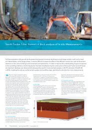
NOTE ON PORE 

PRESSURE 

SOME REMARKS ON PORE PRESSURE 

PARAMETERS A AND B IN UNDRAINED 

ANALYSES WITH THE HARDENING SOIL 

MODEL 

In undrained analyses Skempton’s pore 

pressure parameters A and B (Skempton, 

1954) are frequently used to estimate 

excess pore pressures. If we consider triaxial 

conditions, Skempton’s equation reads 

u = B [ 3 

+ A ( 1 

- 3 

) ] 

where 1 

and 3 

are changes in total minor 

and major principal stresses respectively. For 

fully saturated conditions, assuming pore water 

being incompressible, B is 1.0. Furthermore, 

for elastic behaviour of the soil skeleton, A 

turns out to be 1/3. 

A frequently asked question in PLAXIS courses 

is “What pore pressure parameters A and B does 

PLAXIS use”, if an undrained analysis is 

performed in terms of effective stresses setting 

the material type to undrained? The answer is 

“You don’t know”, except for the trivial cases 

of elastic or elastic-perfectly plastic behaviour. 

In order to investigate this in more detail 

undrained triaxial stress paths are investigated 

with the Mohr Coulomb model with and 

without dilatancy, and with the Hardening Soil 

model. In the latter the influence of various 

assumptions of E 50 

and E oed 

has been studied. 

Soil Parameters 

The following parameter sets have been used 

and the model number given below is referred 

to in the respective diagrams. A consolidation 

pressure of 100 kN/m 2 has been applied to all 

test simulations followed by undrained 

shearing of the sample. 

Pore Pressure Parameter B 

In order to check the value of parameter B in 

an undrained PLAXIS analysis a hydrostatic 

stress state has been applied after 

consolidation. By doing so, the parameter A 

does not come into picture and B can be 

directly calculated from u and 3 

, when 

using undrained behaviour as material type. 

PLAXIS does not yield exactly 1.0 because a 

slight compressibility of water is allowed for 

numerical reasons and therefore a value of 

0.987 is obtained for the given parameters for 

the Mohr Coulomb model. For the HS model 

the value depends slightly on E 50 

and E oed 

, but 

also on the power m and changes with loading. 

The differences however are in the order of 

about 3.0 to 5.0 % for the parameter sets 

investigated here. So it is correct to say that 

Skempton’s pore pressure parameter B is 

approximately 1.0 in PLAXIS, when using 

undrained behaviour as material type. 

Pore Pressure Parameter A 

The value of parameter A is more difficult to 

determine. However one can evaluate A from 

the results of the numerical simulations and 

this has been done for various parameter 

combinations for the Hardening Soil model and 

the Mohr Coulomb model. 

Model Number E ref 50 

E ref ur 

E ref oed 

c ur 

p ref m K nc 0 

R f 

kN/m 2 kN/m 2 kN/m 2 ° ° kN/m 2 - kN/m 2 - - - 

HS_1 30 000 90 000 30 000 35 0 / 10 0.0 0.2 100 0.75 0.426 0.9 

HS_2 50 000 150 000 50 000 35 0 0.0 0.2 100 0.75 0.426 0.9 

HS_3 15 000 45 000 15 000 35 0 0.0 0.2 100 0.75 0.426 0.9 

HS_4 30 000 90 000 40 000 35 0 0.0 0.2 100 0.75 0.426 0.9 

HS_5 30 000 90 000 15 000 35 0 0.0 0.2 100 0.75 0.426 0.9 

HS_6 50 000 150 000 30 000 35 0 0.0 0.2 100 0.75 0.426 0.9 

Parameters for MC Model: E = 30 000 kN/m 2 ; = 0.2; = 35°; = 0° and 10° 

6

PLAXIS 

PLAXIS 

Fig. 1 

Stress path in 

p’-q-space / 

MC – HS model 

Fig. 2 

q- 1 

- diagram / 


Fig. 3 

u- 1 

- diagram / 


Fig. 4 

A- 1 

- diagram / 


parameter A excess pore pressure [kN/m 2 ] q [kN/m 2 ] q [kN/m 2 ] 

Comparison Mohr Coulomb – 

Hardening Soil 

In this comparison we consider the Mohr 

Coulomb criterion and the parameter set 1 for 

the Hardening Soil model for dilatant ( = 10°) 

and non dilatant ( = 0°) behaviour. The p’-qdiagramm 

(Fig. 1) firstly shows that the 

effective stress path observed in a typical 

undrained triaxial test is only obtained for the 

Hardening Soil model because the Mohr 

Coulomb model remains in the elastic range 

and thus no change in effective mean normal 

stress takes place. The well known fact that 

dilatant behaviour leads to an increase of 

strength in the undrained case is reproduced 

by both models in a similar way. It is important 

to point out that although the effective 

strength parameters are the same for both 

models the undrained shear strength is 

different due to different effective stress paths 

produced by both models, the Hardening Soil 

model giving an almost 15% lower value (see 

also Fig. 2). The pore pressure vs vertical strain 

diagram in Fig. 3 shows the expected increase 

of excess pore water pressure followed by a 

rapid decrease for the dilatant material 

behaviour. It is worth noting that in the case 

of the Mohr Coulomb model there is a sharp 

transition when the excess pore water pressure 

starts to decrease (at the point where the 

failure envelope is reached) whereas for the 

Hardening Soil model this transition is smooth. 

The pore pressure parameter A (Fig. 4) is 1/3 

for the non dilatant Mohr Coulomb model (this 

is the theoretical value for elastic behaviour) 

and is independent of the loading stage and 

thus the vertical strain. For the Hardening Soil 

model A is not a constant but increases with 

deviatoric loading to a final value of approx. 

0.44 for this particular parameter set. Of course 

the parameter A tends to become negative for 

dilatant behaviour. 

Hardening Soil – Influence of E ref 50 

and 

E ref oed 

The reference parameter set is HS_1 of Table 

1. Based on this, the reference values of E 50 

and Eoed have been varied (HS_2 to HS_6). Only 

non dilatant material behaviour is considered. 

Fig. 5 shows effective stress paths in the p’-qspace 

and it is interesting to see that for E 50 

= E oed 

the stress path is the same for all values 

of E 50 

leading to the same undrained shear 

strength although the vertical strain (and thus 

the shear strain) at failure is different (Fig. 6). 

If E 50 

is different from E oed 

, different stress 

paths and hence different undrained shear 

7

PLAXIS 

PLAXIS 

Fig. 5 

Stress path in 

p’-q-space / 


Fig. 6 

q- 1 

- diagram / 


Fig. 7 

u- 1 

- diagram / 


Fig. 8 

A- 1 

- diagram / 


parameter A excess pore pressure [kN/m 2 ] q [kN/m 2 ] q [kN/m 2 ] 

strengths are predicted. The difference 

between HS_4 and HS_5 is more than 30% 

which is entirely related to the difference in 

E oed 

. This is perhaps not so suprising because 

E oed 

controls much of the volumetric 

behaviour which in turn is very important for 

the undrained behaviour. However one has to 

be aware of the consequences when using 

these parameters in boundary value problems. 

In Fig. 6 deviatoric stress is plotted against 

vertical strain and – unlike in a drained test 

where E oed 

has only a minor influence on the 

q- 1 

-curve – both parameters have a strong 

influence on the results. E 50 

governs, as 

expected, the behaviour at lower deviatoric 

stresses but when failure is approached the 

influence of E oed 

becomes more pronounced. 

A very similar picture is obtained when excess 

pore pressures are plotted against vertical 

strain (Fig. 7). In Fig. 8 the pore pressure 

parameter A is plotted against vertical strain 

and it follows that for E oed 

> E 50 

(parameter 

set HS_4) the pore pressure parameter A is 

approx. 0.34, i.e. close to the value for elastic 

behaviour. If E oed 

< E 50 

(parameter sets HS_5 

and HS_6) the parameter A increases rapidly 

with loading, finally reaching a value of 

approximately A = 0.6. 

Summary 

It has been shown that the pore pressure 

parameters A and B obtained with PLAXIS from 

undrained analysis of triaxial stress paths using 

a Mohr Coulomb failure criterion are very close 

to the theoretical values given by Skempton 

(1954) for elastic material behaviour, i.e. B is 

approx. 1.0 and A is 1/3. For more complex soil 

behaviour as introduced by the Hardening Soil 

model the parameter A is no longer a constant 

value but changes with loading and is 

dependent in particular on the value of E oed 

in 

relation to E 50 

. For a given E 50 

the parameter 

A at failure is higher for lower E oed 

-values, 

which in turn results in lower undrained shear 

strength. E oed 

< E 50 

is usually assumed for 

normally consolidated clays experiencing high 

volumetric strains under compression which 

corresponds to a higher value for A in the 

undrained case. It is therefore justified to say 

that PLAXIS predicts the correct trend, care 

however has to be taken when choosing E oed 

, 

because the influence of this parameter, which 

may be difficult to determine accurately for in 

situ conditions, is significant and may have a 

strong influence on the results when solving 

practical boundary value problems under 

undrained conditions. 

8

PLAXIS 

PLAXIS 

Fig. 1: 

Surface 

settlements - 

analysis A 

Fig. 2: 

Horizontal 

displacements at 

surface -analysis A 

Fig. 3: 

Displacements of 

slected points - 

analysis A 

Fig. 4: 

Surface 

settlements - 

analysis B 

Fig. 5: 

Horizontal 


surface -analysis B 

horizontal displacements [mm] vertical displacements [mm] displacements [mm] horizontal displacements [mm] vertical displacements [mm] 

Reference 

Skempton, A.W. (1954). The Pore-Pressure 

Coefficients A and B. Geotechnique, 4, 143- 

147. 

H.F. Schweiger 

Graz University of Technology 

Benchmarking I 

PLAXIS BENCHMARK NO.1: SHIELD TUNNEL 

1 - RESULTS 

Introduction 

Unfortunately the response of the PLAXIS 

community to the call for solutions for the 

first PLAXIS benchmark example was not a 

success at all. Probably the example 

specified gave the impression of being so 

straightforward that everybody would 

obtain the same results and thus it would 

not be worthwhile to take the time for this 

exercise. However, I had distributed the 

example on another occasion within a 

different group of people dealing with 

benchmarking in geotechnics. In the 

following I will show the results of this 

comparison together with the few PLAXIS 

results I have got. As mentioned in the 

specification of the problem no names of 

authors or programs are given, so I will not 

disclose which of the analyses have been 

obtained with PLAXIS. 

I hope, that the summary of the first 

benchmark example provides sufficient 

stimulation for taking part in the second call 

for solutions for PLAXIS Benchmark No.2, 

published in this bulletin, so that we can go 

ahead with this section and as awareness for 

necessity of validation procedures grow, 

proceed to more complex examples. The 

specification of Benchmark No.1 is not repeated 

here; please refer to the Bulletin No.11. 

Results Analysis A – elastic, no lining 

Figure 1 shows calculated settlements of the 

9

PLAXIS 

PLAXIS 

Fig. 6: 


selcted points - 

analysis B 

Fig. 7: 

Surface 

settlements - 

analysis C 

Fig. 8: 

Horizontal 


surface analysis C 

Fig. 9: 


selcted points - 

analysis C 

Fig. 10: 

Normal forces and 

contact pressure - 

analysis C 

normal forces [kN]/contact pressure [kPa] displacements [mm] horizontal displacements [mm] vertical displacements [mm] displacements [mm] 

surface and it follows that even in the elastic 

case some scatter in results is observed. 

Some of the discrepancies are due to different 

boundary conditions. ST5, for example, 

restrained vertical and horizontal displacements 

at the lateral boundary, others introduced an 

elastic spring or a stress boundary condition. 

The effect of the lateral boundary is not so 

obvious from Figure 1 but becomes more 

pronounced when Figure 2, showing the 

horizontal displacement at the surface, is 

examined. Figure 3 summarizes calculated 

values at specific points, namely at the surface, 

the crown, the invert and the side wall (for 

exact location see specification). A maximum 

difference of 10 mm (this is roughly 20%) in 

the vertical displacement of point A (at the 

surface) is observed and this is by no means 

acceptable for an elastic analysis. 

Results Analysis B – elastic-perfectly 

plastic, no lining 

Figures 4 and 5 show settlements and 

horizontal displacements at the surface for the 

plastic solution with constant undrained shear 

strength. In Figure 4 a similar scatter as in 

Figure 1 is observed with the exception of ST4, 

ST9 and ST10 which show an even larger 

deviation from the "mean" of all analyses 

submitted. Again ST5 restrained vertical 

displacements at the lateral boundary and thus 

the settlement is zero here. ST9 used a von- 

Mises and not a Tresca failure criterion which 

accounts for the difference. The strong 

influence of employing a von-Mises criterion 

as follows from Figure 4 has been verified by 

separate studies. It is emphasized therefore 

that a careful choice of the failure criterion is 

essential in a non-linear analysis even for a 

simple problem as considered here. The 

significant variation in predicted horizontal 

displacements, mainly governed by the 

placement of the lateral boundary condition, 

is evident from Figure 5. Figure 6 compares 

values for displacements at given points. Taking 

the settlement at the surface above the tunnel 

axis (point A) the minimum and maximum 

value calculated is 76 mm and 159 mm 

respectively. Thus differences are - as expected 

- significantly larger than in the elastic case but 

again not acceptable. 

10

PLAXIS 

PLAXIS 

Fig. 11: 

Surface 

settlements 

analysis A / lateral 

boundary at 100 m 

Fig. 12: 

Horizontal 


surface analysis A 

/ lateral boundary 

at 100 m 

Fig. 13: 

Surface 

settlements 

analysis A / 

undrained - 

drained 

Fig. 14: 

Horizontal 


surface analysis A 

/ undrained - 

drained 

horizontal displacements [mm] vertical displacements [mm] horizontal displacements [mm] vertical displacements [mm] 

Results Analysis C – elastic-perfectly 

plastic, lining and volume loss 

Figure 7 plots surface settlements for the 

elastic-perfectly plastic analysis with a specified 

volume loss of 2% and the wide scatter in 

results is indeed not very encouraging. The 

significant effect of the vertically and 

horizontally restrained boundary condition 

used in ST5 is apparent. However in the other 

solutions no obvious cause for the differences 

could be found except that the lateral 

boundary has been placed at different 

distances from the symmetry axes and that 

the specified volume loss is modelled in 

different ways. Figure 8 shows the horizontal 

displacements at the surface and a similar 

picture as in the previous analyses can be 

found. Figure 9 depicts displacements at 

selected points. The range of calculated values 

for the surface settlement above the tunnel 

axis is between 1 and 25 mm and for the 

crown settlement between 17 and 45 mm 

respectively. The normal forces in the lining 

and the contact pressure between soil and 

lining do not differ that much (variation is 

within 15 and 20% respectively), with the 

exception of ST9 who calculated significantly 

lower values (Figure 10). 

Results with lateral boundary at distance 

of 100 m from tunnel axis 

Due to the obvious influence of the lateral 

boundary conditions a second round of analysis 

has been performed asking all authors to redo 

the analysis with a lateral boundary at 100 m 

distance from the line of symmetry with the 

horizontal displacements fixed. As follows from 

Figures 11 and 12 which depicts these results 

for case A, all results are now within a small 

range and thus it has been confirmed that the 

discrepancies described from the previous 

chapter are entirely caused by the boundary 

condition. In addition to finite element results 

an analytical solution by Verruijt is included for 

comparison. Vertical displacements are in very 

good agreement and also horizontal 

displacements are acceptable in the area of 

interest (i.e. in the vicinity of the tunnel). For 

case B similar results are obtained although 

some small differences are still present. For case 

C the comparison also matches much better 

now but some differences remain here and this 

is certainly due to the fact that the programs 

involved handle the specified volume loss in a 

different way. 

Comparison undrained – drained 

conditions 

In order to show that the influence of the 

lateral boundary is especially important under 

undrained conditions (constant volume) an 

11

PLAXIS 

PLAXIS 

Fig. 1: 

Geometric data 

benchmark excavation 

analysis has been performed for case A with 

exactly the same parameters except for 

Poisson's ratio, chosen now to correspond to 

a drained situation, i.e. deformation under 

constant volume is no longer enforced (for 

simplicity the difference of Young's module 

between drained and undrained conditions has 

been neglected). It follows from Figure 13 that 

for the drained case the surface settlements 

are virtually independent of the distance of the 

lateral boundary (results for mesh widths of 

50 m and 100 m are shown respectively). The 

horizontal displacements (Figure 14) show 

some differences of course but in the area of 

interest they are negligible in the drained case. 

Summary 

The outcome of this benchmark example 

clearly emphasizes the necessity of performing 

these types of exercises in order to improve 

the validity of numerical models. Given the 

discrepancies in results obtained for this very 

simple example much more scatter can be 

expected for real boundary value problems. 

One of the lessons learned from this example 

is that the influence of the boundary 

conditions can be much more severe in an 

undrained analysis than in a drained one and 

whenever possible a careful check should be 

made whether or not the placement of the 

boundary conditions affects the results one is 

interested in. One may argue that this is a trivial 

statement, practice however shows that due 

to time constraints in projects it is not always 

feasible to check the influence of all the 

modelling assumptions involved in a numerical 

analysis of a boundary value problem. It is one 

of the goals of this section to point out 

potential pitfalls in certain types of problems 

which may not be obvious even to experienced 

users and to promote the development of 

guidelines for the use of numerical modelling 

in geotechnical practice. 

Helmut F. Schweiger, Graz University of 

Technology 

Benchmarking II 

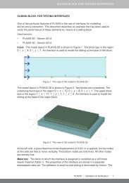
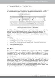
PLAXIS BENCHMARK NO. 2: EXCAVATION 1 

The second benchmark is an excavation in 

front of a sheet pile wall supported by a 

strut. Geometry, excavation steps and 

location of the water table are given in 

Figure 1. Fully drained conditions are 

postulated. The soil is assumed to be a 

homogeneous layer of medium dense sand 

and the parameters for the Hardening Soil 

model, the sheet pile wall and the strut are 

given in Tables 1 and 2 respectively. 

Table 1. 

Parameters for 

sheet pile wall and strut 

EA EI W V 

kN/m kN 2 /m kN/m/m - 

Sheet pile wall 2.52E6 8064 0.655 0.0 

Strut 1.5E6 

The following computational steps have to be 

performed in a plane strain analysis: 

- initial phase (K 0 

= 0.426) 

- activation of sheet pile, excavation step 1 

to level – 2.0 m 

dry 

wet E ref 50 E ref ur E ref oed 

c ur p ref m K nc 0 R f R inter T-Strength 

kN/m 3 kN/m 3 kPa kPa kPa ° ° kPa - kPa - - - - kPa 

19.0 20.0 45 000 180 000 45 000 35 5 1.0 0.2 100 0.55 0.426 0.9 0.7 0.0 

Table 2. Parameters for HS-model 

12

PLAXIS 

PLAXIS 

- activation of strut at level –1.50 m, 

excavation step 2 to level – 4.0 m, 

- groundwater lowering inside excavation to 

level – 6.0 m 

- excavation step 3 to level – 6.0 m 

- phi-c-reduction 

REQUIRED RESULTS 

1. bending moments and lateral deflections of 

sheet pile wall (including values given in a 

table) 

2. surface settlements behind wall (including 

values given in a table) 

3. strut force 

4. factor of safety obtained from phi-creduction 

for the final excavation step 

Note: As far as possible results should be 

provided not only in print but also on disk 

(preferably EXCEL) or in ASCII-format respectively. 

Alternatively, the entire PLAXIS-project may be 

provided. Results may also be submitted via e- 

mail to the address given below. 

Results should be sent no later than 

August 1st, 2002 to: 

Prof. H.F. Schweiger 

temporary occupied the chair on behalf of 

MOS Grondmechanica BV. 

Since the very beginning Dr. Bakker has been 

actively involved in the program(ming) of 

PLAXIS and is a key figure in the PLAXIS 

network. In his last position he was Head of 

Construction and Development at the Tunnelengineering 

department for the Dutch Ministry 

of Public Works. Furthermore he is a lecturer 

at Delft University of Technology. 

COURSES 

In 2001 over 400 people attended one of 

the 13 Plaxis courses that were held in 

several parts of the world. Most of these 

courses are held on a regular basis, while 

others take place on an single basis. 

Institute for Soil Mechanics and Foundation 

Engineering 

Computational Geotechnics Group 

Graz University of Technology 

Rechbauerstr. 12, A-8010 Graz 

Tel.: +43 (0)316 – 873-6234 

Fax: +43 (0)316 – 873-6232 

E-mail: schweiger@ibg.tu-graz.ac.at 

http://www.tu-graz.ac.at/geotechnical_group/ 

Recent Activities 

NEW DIRECTOR OF PLAXIS B.V. 

We are pleased to introduce the new 

director of PLAXIS BV, Dr. Klaas Jan Bakker. 

Dr. Bakker who started the first of February 

takes over the chair of Mr. Hutteman, who 

Regular courses: 

Traditionally, we start the year with the standard 

International course “Computational 

Geotechnics” that takes place during the 3rd 

week of January in the Netherlands. The 

Experienced users course in the Netherlands 

is traditionally organised during the 4th week 

of March each year. Besides these standard 

courses in the Netherlands, some other regular 

courses are held in Germany (March), England 

(April), France (Autumn), Singapore (Autumn), 

Egypt, and the USA. For the USA the course 

schedule is a bit different, as we plan to have 

an Experienced users course per two years and 

two standard courses in the intermediate 

periods. In May, 2002, we had the Experienced 

users course in Boston, which was organised 

in cooperation with the Massachusetts Institute 

of Technology (MIT). For January 2003, a 

standard course is scheduled in Berkeley in 

13

PLAXIS 

PLAXIS 

cooperation with the University of California. 

For August, 2003, another standard course is 

organised in Boulder in cooperation with the 

University of Colorado. It is our intention to 

repeat this scheme of courses for the Western 

hemisphere. For the Asian region, we have 

planned a similar schedule that also includes 

an experienced users course once every two 

years. 

Other courses: 

Besides the above regular courses, other 

courses are organised in different parts of the 

world. In the past year, courses were held in 

Mexico, Vietnam, Turkey, Malaysia, etc. On the 

last page of this bulletin, you can see the 

agenda, which lists all scheduled courses and 

some other events. Our web-site www.plaxis.nl 

on the other hand will always give you the 

most up-to-date information. 

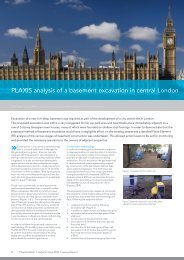
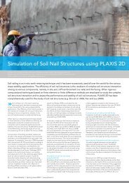
PLAXIS Practice I 

1. Introduction 

In Würenlingen (Switzerland), for the 

temporary storage of nuclear waste, an 

extension of the existing depository was 

required. To facilitate this, a 7.5 - 9.0 m deep 

excavation was necessary. This bordered 

immediately adjacent pre-existing 

structures. Furthermore, along one of it‘s 

sides there is a route used for the 

transportation of nuclear waste. 

Photo 1: 

Participants in the 

Experienced users 

course, March 2002, the 

Netherlands. 

2. Project 

Length of excavation: 98 m 

Width of excavation: 33 m 

Maximum depth: 9 m 

Start of works: Spring 2001 

End of construction: Summer 2001 

Photo 2: 

Plaxis short course, 

October 2001, Mexico 

3. Geotechnical conditions 

In the Würenlingen area, significant deposits 

of the Aare River dominate, which comprises 

predominantly gravels and sands. The 

groundwater table lies at a depth of ca. 9.5 m 

below the surface prior to excavation. The 

gravels and sands are known as good 

foundation material, with some low apparent 

cohesion, allowing for the temporary 

construction of vertical cuttings of low height. 

Photo 3: 

Plaxis short course, 

November 2001, 

Vietnam. 

4. Construction procedure 

Due to space restrictions, a sloped earthworks 

profile is not possible. Therefore, it was 

concluded to undertake the excavation using 

Model Behavior unsat 

sat 

E ref 50 

E ref oed 

m E ref ur 

ur 

c R inter 

- kN/m3 kN/m3 kPa kPa - KPa - kPa ° ° - 

HS Drained 22.0 22.0 33 000 37 500 0.5 99 000 0.25 1.0 32 6 1.0 

Table 1. Soil parameters 

14

PLAXIS 

PLAXIS 

Fig. 1: 

Typical section 

with horizontal 

displacements 

a soil nailing option. Correspondingly, the 

excavation had to proceed in benched stages. 

Each bench had a height of 1.30 m and a width 

of 4.5 to 6.0 m. The free face was immediately 

covered with an 18 cm thick layer of shotcrete 

and tied back with untensioned soil nails. 

The bond strength of the soil nails was 

established by pullout tests. Usually the soil 

nails are cemented along their full length. For 

the pullout tests, however, the bond length 

was reduced to between 3.0 and 4.0 m with a 

total length of 7.0 m. The individual nails have 

a cross-sectional area of 25 mm and yield 

strength of 246 kN. During the pullout tests, 

it was possible to tension the nails to yield point 

without any indication of creep or failure. 

In total five benches were necessary to reach 

excavation depth. The wall itself is vertical, with 

nail spacing of 1.5 m and 1.3 m, horizontal and 

vertical respectively. The nails were tightened 

three days after installation with a torque key, 

to secure a fast seat to the shotcrete. A pretensioning 

with fully cemented nails is not 

sensible (see fig. 1). 

5. Calculations 

The initial calculations were performed with 

the usual statical programs based on beam 

theory and limiting equilibrium loading. Due 

to the particular safety requirements in 

connection with nuclear transport additional 

deformation predictions were made. These 

calculations were carried out with Plaxis version 

7. Geotextile elements were used to model the 

nails. Due to the good bonding of the soil nails 

proven by the pullout attempts, no reduction 

was made for loading transfer along the 

geotextile elements. 

The calculations were performed with the 

following parameters: 

● Hardening soil model 

● Plane strain with 6 node elements 

● 649 elements 

● Due to the simple geology, only one soil layer 

was used (see table 1) 

● Due to good bonding between soil and 

shotcrete wall no reduction in interface 

friction was made. 

● The calculations were performed without 

groundwater. 

● Shotcrete wall of 18 cm thickness with 

reinforced wire mesh, modeled as beam 

elements. EA = 5.4 x 10 6 kN/m, EI = 

1.458 x 104 kNm 2 /m and = 0.2 

● Soil nails are modeled as geotextile elements. 

EA = 6.87 x 10 4 kN/m and = 0. 

● Results 

Final excavation stage 

Maximum deformation of shotcrete wall; 

17 mm (see fig. 2a and fig. 3). 

Maximum horizontal deformation of 

shotcrete wall; 14 mm (see fig. 2d). 

Maximum force in geotextile element; 49 

kN/m, or 73.5 kN per nail (see fig. 4). 

Maximum bending moment in shotcrete 

wall; 11.5 kNm/m (see fig. 2b). 

Maximum axial force in shotcrete wall; -67 

kN/m (see fig. 2c). 

It must be noted, that the tensile forces in the 

geotextile elements at the final excavation 

stage did not calculate to zero at the toe of 

the nail, as should be in reality. This could be 

due to a too wide FE-net around the geotextile 

elements, additionally due to the use of only 

6-nodes instead of the more precise 15-node 

element. 

6. Measurement on site 

In total, deformation of the excavation was 

taken at five stations. Prior to excavation 

clinometers were placed ca. 1.0 m behind the 

proposed shotcrete wall, with a depth of 7 m 

below excavation level. Figure 7 shows the 

measured horizontal deformations of two 

cross-sections with equal depths (7.2 and 9.0 

mm). Figure 6 contains the calculated 

horizontal deformations along a vertical line 

15

PLAXIS 

PLAXIS 

Fig. 2: 

Output in 

shotcrete wall 

Fig. 3: 

Deformation of 

geotextile 

1m behind the shotcrete wall (14.9 mm). A 

comparison shows that the calculated 

deformations are greater than the measured. 

Conspicuous is, that below the excavation base 

there is practically no movement measurable. 

Plaxis, however, has predicted some 4 mm 

deformation. This may be due to an initial 

offset or due to stiffer behavior at the bottom 

of the excavation. 

The maximum measured horizontal 

deformation was between 7.2 and 9.0 mm at 

the wall head. Plaxis calculated 14.9 mm 

horizontal deformation at this point. 

If only relative measurements are considered, 

assuming that no movement takes place at the 

wall toe, then the prediction from Plaxis lays 

very close to the actual maximum measured. 

The forms of the measured and calculated 

deformation curves correspondwell well with 

each other. 

Fig. 4: 

Axial Forces in 

geotextile 

7. Conclusions 

The calculated deformation of the nailed wall 

corresponds well with the measured values, 

especially if the predicted deformations of 

Plaxis below excavation level are not 

considered. 

The soil parameters used correspond to 

conservative average values, evaluated from a 

large number of previous sites under similar 

conditions. It is plausible that the deformation 

parameters are underestimated. 

Fig. 5: 

Measured 

displacements 

Fig. 6: 

Calculated 

displacement 

The Plaxis calculation illustrates 

comprehensively, that the soil nailing system 

(soil-nail-wall) works as an interactive system. It 

shows further, that the maximum nail force 

does not necessarily act at the nail head, but 

according to the distribution of soil movements 

may also lie far behind the head of the nail. This 

means that displacements are necessarily taking 

place before the nail force is activated. 

On the one hand, it shows that the shotcrete 

wall in vertical alignment is stressed by bending 

and compression, and that the wall’s foot 

transmits compressive stresses to the soil. On 

the other hand, the shotcrete wall in horizontal 

alignment is only loaded by bending, whereby 

in the absence of lateral restrictions of 

deformation there could also be tension. Finally 

it is clear to see, that nail head support and 

pullout failure should be considered (see fig. 4). 

16

PLAXIS 

PLAXIS 

Thanks to prior deformation calculation with 

Plaxis and measurement control by clinometer 

installation during the construction stage, the 

safety of the works in relation to nuclear 

transportation could be assessed at all times. 

H.J. Gysi, G.Morri, Gysi Leoni Mader AG, 

Zürich - Switzerland 

● 

Calculation procedure 

Phase 1: Initial stresses, using Mweight = 1. 

Phase 2: Live load (5 kN/m 2 and 10 kN/m 2 ) 

Phase 3: Excavation to top level of 

wall (-0.80 m). 

Phase 4: First excavation stage, 

including shotcrete of wall 

and installation of first row 

of soil nails (-2.10 m). 

Phase 5: Second excavation stage with 

shotcrete wall (-3.40 m). 

Phase 6: Installation of second row 

of soil nails. 

Phase 7: Third excavation stage 

with shotcrete wall (-4.70 m). 

Phase 8: Installation of third row of soil nails. 

Phase 9: Fourth excavation stage 


Phase 10: Installation of fourth row 

of soil nails. 

Phase 11: Fifth excavation stage 


Phase 12: Installation of fifth row of soil nails. 

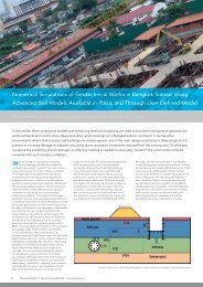
PLAXIS Practice II 

FINITE ELEMENT MODELLING OF A DEEP 

EXCAVATION SUPPORTED BY JACK-IN 

ANCHORS 

filled layer of very loose silty sand and very soft 

peaty clay varies from 11m to 13m. Due to the 

presence of very soft soil condition and the 

fast track requirement of the project, 

Contiguous Bored Pile (CBP) walls supported 

by soil nails were used to support the 

excavation process. This hybrid technique was 

envisaged and implemented due to its speed 

in construction and the ability of the Jack-in 

Anchors 1) in supporting excavations in 

collapsible soils, high water table and in soft 

soils conditions (Cheang et al., 1999 & 2000, 

Liew et al, 2000). The use of soil nailing in 

excavations and slope stabilisation has gained 

wide acceptance in Southeast Asia, specifically 

in Malaysia and Singapore due to its 

effectiveness and huge economic savings. 

Adopting the observational method, numerical 

analyses using ‘PLAXIS version 7.11’ a finite 

element code were conducted to study the 

soil-structure interaction of this relatively new 

retaining system. Numerical predictions were 

compared with instrumented field readings and 

deformation parameters were back analysed 

and were used in subsequent prediction of wall 

movements in the following excavation stages. 

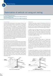
2. SUBSURFACE GEOLOGY 

The general subsurface soil profile of the site, 

shown in Table 1 consists in the order of 

succession of loose clayey SILT, loose to 

medium dense Sand followed by firm to hard 

clayey SILT. The residual soils (Figure 1) are interlayered 

by 9m thick soft dark peaty CLAY. For 

analysis purposes the layers were simplified 

1) Jack-in Anchor Technique is a patented 

product by Specialist Grouting Engineers 

Sdn. Bhd. Malaysia 

1. INTRODUCTION 

A mixed development project that is located 

at UEP Subang Jaya, Malaysia consists of three 

condominium towers of 33 storeys and a single 

20-storey office tower. Due to the huge 

demand for parking space, an approximately 

three storey deep vehicular parking basement 

was required. The deep excavation, through a 

Photo 1: Jack-in Anchor Technique 

17

PLAXIS 

PLAXIS 

into representative granular non-cohesive and 

cohesive material, such as: 

Photo 2: 

The Retaining System: 

Contiguous Bored Pile 

Wall Supported by Jackin 

Anchors that function 

as Soil Nails 

DEPTH (m) DESCRIPTION SPT ‘N’ VALUE 

LAYER 1 0 to 9 Clayey SILT 18 

LAYER 4 27 to 35 Dense SILT >50 

Fig. 1: 

Typical Subsurface Profile 

Table 1. Soil Layers 

3. THE RETAINING SYSTEM 

In view of the close proximity of commercial 

buildings to the deep excavation, a very stiff 

retaining system is required to ensure minimal 

ground movements the retained side of the 

excavation. Contiguous Bored Pile that acts as 

an earth retaining wall during the excavation 

works were installed along the perimeter of 

the excavation and supported by jack-in 

anchors. The retaining wall system consist of 

closely spaced 1000mm diameter contiguous 

bored piles supported by hollow pipes which 

functions as soil nails are installed by hydraulic 

jacking using the Jacked-in Soil Anchor 

Technology as shown in photo 3. Figure 2 

illustrates the soil nail supported bored pile wall 

system. 

Fig. 2a: 

The Retaining System 

Photo 3: 

Hydraulic Jacking 

Fig. 2b: 

The Retaining System 

18

PLAXIS 

PLAXIS 

Fig. 4: 

Geotechnical 

Instruments 

This method has proven to be an efficient and 

effective technique for excavation support, 

where conventional soil nails and ground 

anchors have little success in such difficult soft 

soil conditions. Such conditions are sandy 

collapsible soil, high water table and in very 

soft clayey soils where there is a lack of shortterm 

pullout resistance. 

Relatively, larger movements are required to 

mobilise the tensile and passive resistance of 

the jacked-in pipes when compared to ground 

anchors. However it was anticipated that the 

ground settlement at the retained side and 

maximum lateral displacement of the wall 

using this system would still be within the 

conditions and the close proximity of the 

commercial buildings to the deep excavation, 

a performance monitoring program was 

provided. Firstly, as a safety control. Second, 

to refine the numerical analysis using field 

measurements obtained at the early stages of 

construction and third, to provide an insight 

into the possible working mechanisms of the 

system. 

The geotechnical instrumentation program 

consists of 18 vertical inclinometer tubes 

located strategically along the perimeter 

within the Contiguous Bored Pile wall and 30 

optical survey makers (surface settlement 

points) near the vicinity of the commercial 

buildings. The locations of these instruments 

are detailed in Fig. 4 for the inclinometers. 

Fig. 5 illustrates the restrained trend of 

horizontal displacement of the wall as 

measured through inclinometers installed at 

the site 

Fig. 5: 

Measures deflection 

profile 

required tolerance after engineering 

assessment. 

4. GEOTECHNICAL INSTRUMENTATION 

In view of this relatively new excavation 

support technique used for in-situ soft soil 

5. FINITE ELEMENT MODELLING 

EQUIVALENT PLATE MODEL 

Equivalence relationships have to be developed 

between the 3D structure and 2D numerical 

model. Non 2-D member such as soil nails must 

be represented with ‘equivalent’ properties that 

reflect the spacing between such elements. 

Donovan et al. (1984) suggested that properties 

of the discrete elements could be distributed 

over the distance between the elements in a 

19

PLAXIS 

PLAXIS 

uniformly spaced pattern by linear scaling. 

Unterreiner et al. (1997) adopted an approach 

similar to Al-Hussaini and Johnson (1978) where 

an equivalent plate model replaces the discrete 

soil-nail elements by a plate extended to full 

width and breadth of the retaining wall. Nagao 

and Kitamura (1988) converted the properties 

of the 3-D discrete elements into an equivalent 

composite plate model by taking into account 

the properties of the adjacent soil. The twodimensional 

finite element analysis performed 

hereafter uses the ‘composite plate model’ 

approach. 

Fig 6: 

2-Dimensional finite element mode 

Finite Element Analysis 

The finite element analyses were performed 

using ‘PLAXIS’ (Brinkgreve and Vermeer, 1998). 

The Contiguous Bored Pile wall and steel tubes 

were modelled using a linear-elastic Mindlin 

plate model (Figure 6). The nails were ‘pinned’ 

to the CBP wall. The soil-nail soil interface was 

modelled using the elastic-perfectly-plastic 

model where the Coulomb criterion 

distinguishes between the small displacement 

elastic behaviour and ‘slipping’ plastic behaviour. 

Figure 7: 

E CONC. 

2.00E+07 kN/m 2 element prediction (Prediction No.1) based on 

The surrounding soils were modelled using the 

Lateral Deflection of Soil Nailed 

Contiguous Bored Pile Wall 

Mohr-Coulomb soil model. Table 2 and 3 shows 

the properties used for the analyses. 

6. COMPARISON OF FIELD INSTRUMENTED 

AND PREDICTED DISPLACEMENT READINGS 

Measured And Predicted Lateral Deflection 

Figure 7 compares the in-situ, predicted and 

back analysed lateral deflection of the soil nail 

supported wall. The measured lateral deflection 

Table 2: Soil Properties 

Layer 1 Layer 2 Layer 3 Layer 4 

E (kN/m 2 ) 34000 9000 30000 200000 

soil 

(kN/m 3 ) 19 20 20 19 

0.25 0.25 0.25 0.25 

25 0 35 30 

Figure 8: 

C 2 12 2 2 

Lateral Deflection of ‘Stiff’ and ‘Flexible’ 

Soil Nail System 

0 0 0 0 

is showing a trend of restrained cantilever and 

Table 3: Nail and Contiguous Bored Pile Wall Properties 

the jack-in anchors are restraining the 

E NAIL 

2.90E+06 kN/m 2 

horizontal displacement of the wall. Initial finite 

soil strengths correlated from laboratory 

20

PLAXIS 

PLAXIS 

Figure 9: Influence of 

Nail Stiffness 

results. Excavation involves mainly the 

unloading of adjacent soil, the ground stiffness 

is dependent on stress level and wall 

movements. These aspects were taken into 

account in prediction no.2, the trend is similar 

and a better prediction was obtained. 

Subsequent finite element runs were made 

base on the improved parameters. 

system. Soil-nail lateral resistance is dependent 

not only on the relative stiffness and yield 

strengths of the soil and nail, but also on the 

local lateral displacement across the shear zone. 

Due to the hybrid nature of this system, the 

results indicated that the relative stiffness of 

the nail and wall too governs the development 

of bending i.e., lateral resistance of the soil nail. 

In soft soils, numerical results indicated greater 

bending moments in the nails due to larger wall 

deflection. The implication of this study is 

additional analysis of different working 

mechanisms in various soil types should be 

envisaged. 

7. SOIL-NAIL-SOIL-STRUCTURE 

INTERACTION 

Lateral Bending Stiffness of Soil Nails 

A flexible nail system with a bending stiffness 

of 1/220 of the stiff nail system was numerically 

simulated. It was hypothesised that if bending 

stiffness of the inclusions were insignificant in 

the performance of the nail system, there 

would be no difference in the lateral 

displacement of the wall. However figure 8 

shows that bending stiffness is significant, at 

least in a soil nail supported embedded wall. 

With a stiff nail system, the lateral displacement 

was significantly reduced. Figure 9 illustrates 

that the influence increases as excavation 

proceeds further, this is due to the fact that 

larger movements are required to mobilised 

lateral bending resistance of the nails. 

8. CONCLUSION 

The soil-nail-soil-structure interaction of a nailed 

wall is complex in nature. Soil nails are subjected 

to tension, shear forces and bending moments. 

The outcome of this numerical investigation of 

a real soil-nailed supported Contiguous Bored 

Pile wall in soft residual soils is that nail bending 

stiffness has a significant effect as deformation 

progresses, at least in this hybrid support 

9. REFERENCE 

1. Al-Hussaini, M.M., Johnson, L., (1978), 

Numerical Analysis of Reinforced Earth Wall, 

Proc. Symp. On Earth Reinforcement ASCE 

Annual Convention, p.p. 98-126. 

2. Brinkgreve, R.B.J., Vermeer, P.A., (1998), 

Plaxis- Finite Element Code for Soil and Rock 

Analyses- Version 7.11,A.A.Balkema. 

3. Cheang, W.L., Tan, S.A., Yong, K.Y., Gue, S.S,, 

Aw, H.C., Yu, H.T., Liew, Y.L., (1999), Soil Nailing 

of a Deep Excavation in Soft Soil, 

Proceedings of the 5Th International 

Symposium on Field Measurement in 

Geomechanics, Singapore, Balkema. 

4. Cheang, W.L., Luo, S.Q., Tan, S.A., Yong, Y.K., 

(2000), Lateral Bending of Soil Nails in an 

Excavation, International Conference on 

Geotechnical & Geological Engineering, 

Australia. ( To be Published) 

5. Donovan, K., Pariseau, W.G., and Cepak, 

M.,(1984), Finite Element Approach to Cable 

Bolting in Steeply Dipping VCR Slopes, 

Geomechanics Application in Underground 

Hardrock Mining, pp.65-90.New York: Society 

of Mining Engineers. 

6. Liew, S.S., Tan, Y.C., Chen, C.S., (2000), Design, 

Installation and Performance of Jack-In-Pipe 

Anchorage System For Temporary Retaining 

Structures, International Conference on 

Geotechnical & Geological Engineering, 

Austraila. ( To be Published) 

7. Nagao, A., Kitamura, T., (1988), Filed 

Experiment on Reinforced Earth and its 

Evaluation Using FEM Analysis, International 

21

PLAXIS 

PLAXIS 

Symposium on Theory and Practice of Earth 

Reinforcement, Japan, pp.329-334. 

8. Unterreiner, P., Benhamida, B., Schlosser, F., 

(1997), Finite Element Modelling Of The 

Construction Of A Full-Scale Experimental Soil- 

Nailed Wall. French National Research Project 

CLOUTERRE, Ground Improvement, p.p. 1-8. 

W.L.Cheang, Research Scholar, 

E-mail: engp9168@nus.edu.sg, 

S.A.Tan, Associate Professor, 

E-mail: cvetansa@nus.edu.sg, 

Modelling a row of piles or a row of grout 

bodies in the z-direction can be done by 

dividing the EA real 

and EL real 

by 

the centre-to-centre distance Ls. 

For a beam: 

EA real 

=E real 

*d real 

*b real 

[kN] 

EA plaxis 

= EA real 

/Ls [kN/m] 

For a grout body: 

EA real 

=E real 

*d real 

*b real 

[kN] 

EA plaxis 

= EA real 

/Ls [kN/m] 

K.Y.Yong, Professor, Department of Civil 

Engineering, National University of 

Singapore 

Users Forum 

BEAM TO PILE PROPERTIES 

IN PLAXIS 

Properties for anchors are entered per anchor 

so : EA = [kN] per anchor 

Ls = [m] is spacing centre to centre 

Fig 1. 

Partial geometry 

for shieldtunnel 

project 

Beams and geotextiles are continuous in the 

z-direction (perpendicular to the screen). 

Therefore, a beam /geotextile will be a 

continuous plate/textile in the z-direction. The 

properties are entered per meter 

in the z-direction EA = [kN/m], EL = [kN/m 2 /m] 

Some geometries 

In the past bulletins, a few articles were related 

to experience with the 3D Tunnel program. 

Since it’s release last year, the 3D Tunnel 

program has been used in practice for some 

interesting projects. In the below graphs, 

without further explanation you will find a brief 

overview of possible projects and geometries. 

The printed figures also indicate that the 3D 

Tunnel program can deal with projects beyond 

tunneling. 

22

PLAXIS 

PLAXIS 

Fig 2. Partial 

geometry for pileraft 

foundation 

Fig 3. 

Displacement 

contours for shield 

tunnel project 

Fig 4. 

Partial geometry for anchored retaining wall. 

Fig 5. 

Deformed mesh for interacting tunnels. 

23

PLAXIS 

PLAXIS ACTIVITIES 

8-10 MAY, 2002 

International course for experienced Plaxis users 

(English) 

Boston, USA 

19-22 JANUARY, 2003 

Short course on Computational Geotechnics 

(English) 

Noordwijkerhout, The Netherlands 

16 MAY, 2002 

2nd French Plaxis Users meeting (French) 

Paris, France 

14-18 OCTOBER, 2002 


(Arabic, English) 

Cairo, Egypt 

25-26 OCTOBER, 2002 


(Portuguese, English) 

Sao Paulo, Brazil 

7-8 NOVEMBER, 2002 

11th European Plaxis Users meeting (English) 

Karlsruhe, Germany 



(English) 

Trondheim, Norway 



(French) 

‘Pratique des éléments finis en Géotechnique’ 

Paris, France 

6-9 JANUARY, 2003 

Short course on Computational Geotechnics & 

dynamics (English) 

Berkeley, USA 

10-12 MARCH, 2003 


(German) 

Stuttgart, Germany 

23-26 MARCH, 2003 

International course for experienced Plaxis users 

(English) 

Noordwijkerhout, The Netherlands 

8-10 APRIL, 2003 


(English) 

Manchester, England 

28-30 APRIL, 2003 


(Italian) 

Napoli, Italy 

31 JULY–2 AUGUST, 2003 

Experienced Plaxis users course (English) 

Singapore 

For more information on these activities 

please contact: 

PLAXIS bv 

P.O. Box 572 

2600 AN DELFT 

The Netherlands 

Tel: +31 15 26 00 450 

Fax: +31 15 26 00 451 

E-mail: info@plaxis.nl 

24

Bulletin 12, Summer 2002 - Plaxis

Create successful ePaper yourself

Delete template?

Save as template?