- Page 2:
This page intentionally left blank
- Page 8:
Computability and Logic Fifth Editi
- Page 12:
For SALLY and AIGLI and EDITH
- Page 18:
viii CONTENTS BASIC METALOGIC 9 APr
- Page 24:
Preface to the Fifth Edition The or
- Page 28:
PREFACE TO THE FIFTH EDITION xiii T
- Page 36:
1 Enumerability Our ultimate goal w
- Page 40:
1.1. ENUMERABILITY 5 we might have
- Page 44:
1.2. ENUMERABLE SETS 7 member of A,
- Page 48:
1.2. ENUMERABLE SETS 9 The pair (m,
- Page 52:
1.2. ENUMERABLE SETS 11 a pair G(n)
- Page 56:
1.2. ENUMERABLE SETS 13 on Example
- Page 60:
PROBLEMS 15 the set of all positive
- Page 64:
DIAGONALIZATION 17 supposition must
- Page 68:
DIAGONALIZATION 19 has that much ti
- Page 72:
PROBLEMS 21 2.4 Show that the set o
- Page 76:
3 Turing Computability A function i
- Page 80:
TURING COMPUTABILITY 25 carried out
- Page 84:
TURING COMPUTABILITY 27 in general
- Page 88:
TURING COMPUTABILITY 29 It will the
- Page 92: TURING COMPUTABILITY 31 But if ther
- Page 96: TURING COMPUTABILITY 33 A numerical
- Page 100: 4 Uncomputability In the preceding
- Page 104: 4.1. THE HALTING PROBLEM 37 machine
- Page 108: 4.1. THE HALTING PROBLEM 39 Turing
- Page 112: 4.2. THE PRODUCTIVITY FUNCTION 41 g
- Page 116: 4.2. THE PRODUCTIVITY FUNCTION 43 F
- Page 120: 5 Abacus Computability Showing that
- Page 124: 5.1. ABACUS MACHINES 47 be thought
- Page 128: 5.1. ABACUS MACHINES 49 Figure 5-4.
- Page 132: 5.2. SIMULATING ABACUS MACHINES BY
- Page 136: 5.2. SIMULATING ABACUS MACHINES BY
- Page 140: 5.2. SIMULATING ABACUS MACHINES BY
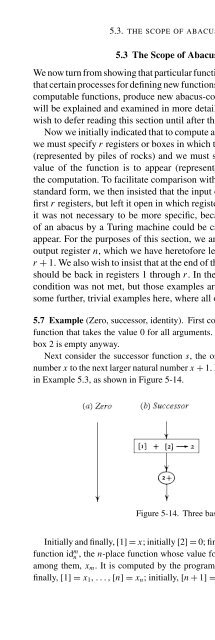
- Page 146: 58 ABACUS COMPUTABILITY Three diffe
- Page 150: 60 ABACUS COMPUTABILITY Figure 5-16
- Page 154: 62 ABACUS COMPUTABILITY 5.7 Show th
- Page 158: 64 RECURSIVE FUNCTIONS (including z
- Page 162: 66 RECURSIVE FUNCTIONS Similarly, f
- Page 166: 68 RECURSIVE FUNCTIONS To put these
- Page 170: 70 RECURSIVE FUNCTIONS Proofs Examp
- Page 174: 72 RECURSIVE FUNCTIONS 6.3 Show tha
- Page 178: 74 RECURSIVE SETS AND RELATIONS dec
- Page 182: 76 RECURSIVE SETS AND RELATIONS whi
- Page 186: 78 RECURSIVE SETS AND RELATIONS Pro
- Page 190: 80 RECURSIVE SETS AND RELATIONS whe
- Page 194:
82 RECURSIVE SETS AND RELATIONS (b)
- Page 198:
84 RECURSIVE SETS AND RELATIONS 7.2
- Page 202:
86 RECURSIVE SETS AND RELATIONS so
- Page 206:
8 Equivalent Definitions of Computa
- Page 210:
90 EQUIVALENT DEFINITIONS OF COMPUT
- Page 214:
92 EQUIVALENT DEFINITIONS OF COMPUT
- Page 218:
94 EQUIVALENT DEFINITIONS OF COMPUT
- Page 222:
96 EQUIVALENT DEFINITIONS OF COMPUT
- Page 226:
98 EQUIVALENT DEFINITIONS OF COMPUT
- Page 232:
9 APrécis of First-Order Logic: Sy
- Page 236:
9.1. FIRST-ORDER LOGIC 103 The nonl
- Page 240:
9.1. FIRST-ORDER LOGIC 105 (For the
- Page 244:
9.2. SYNTAX 107 Thus the more or le
- Page 248:
9.2. SYNTAX 109 notation as the off
- Page 252:
9.2. SYNTAX 111 given formula to be
- Page 256:
PROBLEMS 113 9.3 Consider a languag
- Page 260:
10.1. SEMANTICS 115 The atomic sent
- Page 264:
10.1. SEMANTICS 117 yields two. So
- Page 268:
10.2. METALOGICAL NOTIONS 119 is tr
- Page 272:
10.2. METALOGICAL NOTIONS 121 (the
- Page 276:
PROBLEMS 123 can be said in a first
- Page 280:
PROBLEMS 125 10.14 Show that the fo
- Page 284:
11.1. LOGIC AND TURING MACHINES 127
- Page 288:
11.1. LOGIC AND TURING MACHINES 129
- Page 292:
11.1. LOGIC AND TURING MACHINES 131
- Page 296:
11.2. LOGIC AND PRIMITIVE RECURSIVE
- Page 300:
PROBLEMS 135 the decision problem f
- Page 304:
12 Models A model of a set of sente
- Page 308:
12.1. THE SIZE AND NUMBER OF MODELS
- Page 312:
12.1. THE SIZE AND NUMBER OF MODELS
- Page 316:
12.2. EQUIVALENCE RELATIONS 143 Nam
- Page 320:
12.2. EQUIVALENCE RELATIONS 145 b i
- Page 324:
12.3. THE LÖWENHEIM-SKOLEM AND COM
- Page 328:
PROBLEMS 149 of completeness shows
- Page 332:
PROBLEMS 151 12.12 Show that if two
- Page 336:
13 The Existence of Models This cha
- Page 340:
13.1. OUTLINE OF THE PROOF 155 13.3
- Page 344:
13.3. THE SECOND STAGE OF THE PROOF
- Page 348:
13.3. THE SECOND STAGE OF THE PROOF
- Page 352:
13.4. THE THIRD STAGE OF THE PROOF
- Page 356:
13.5. NONENUMERABLE LANGUAGES 163 w
- Page 360:
PROBLEMS 165 13.11 Let A be a sente
- Page 364:
14.1. SEQUENT CALCULUS 167 equivale
- Page 368:
14.1. SEQUENT CALCULUS 169 We natur
- Page 372:
14.1. SEQUENT CALCULUS 171 conditio
- Page 376:
14.9 Example. Proper use of the two
- Page 380:
14.2. SOUNDNESS AND COMPLETENESS 17
- Page 384:
14.2. SOUNDNESS AND COMPLETENESS 17
- Page 388:
14.3. OTHER PROOF PROCEDURES AND HI
- Page 392:
14.3. OTHER PROOF PROCEDURES AND HI
- Page 396:
14.3. OTHER PROOF PROCEDURES AND HI
- Page 400:
PROBLEMS 185 unformalized mathemati
- Page 404:
15 Arithmetization In this chapter
- Page 408:
15.1. ARITHMETIZATION OF SYNTAX 189
- Page 412:
15.1. ARITHMETIZATION OF SYNTAX 191
- Page 416:
Table 15-2. Gödel numbers of symbo
- Page 420:
15.2. GÖDEL NUMBERS 195 Now s is t
- Page 424:
PROBLEMS 197 where the presence of
- Page 428:
16 Representability of Recursive Fu
- Page 432:
16.1. ARITHMETICAL DEFINABILITY 201
- Page 436:
16.1. ARITHMETICAL DEFINABILITY 203
- Page 440:
16.1. ARITHMETICAL DEFINABILITY 205
- Page 444:
16.2. MINIMAL ARITHMETIC AND REPRES
- Page 448:
16.2. MINIMAL ARITHMETIC AND REPRES
- Page 452:
16.2. MINIMAL ARITHMETIC AND REPRES
- Page 456:
Another example is the proof of the
- Page 460:
16.3. MATHEMATICAL INDUCTION 215 Am
- Page 464:
PROBLEMS 217 and then second z ′
- Page 468:
PROBLEMS 219 relation < 1 of Proble
- Page 472:
17.1. THE DIAGONAL LEMMA AND THE LI
- Page 476:
17.1. THE DIAGONAL LEMMA AND THE LI
- Page 480:
17.2. UNDECIDABLE SENTENCES 225 Suc
- Page 484:
17.3*. UNDECIDABLE SENTENCES WITHOU
- Page 488:
17.3*. UNDECIDABLE SENTENCES WITHOU
- Page 492:
PROBLEMS 231 every axiom of Q is a
- Page 496:
THE UNPROVABILITY OF CONSISTENCY 23
- Page 500:
THE UNPROVABILITY OF CONSISTENCY 23
- Page 504:
HISTORICAL REMARKS 237 From (2) and
- Page 508:
HISTORICAL REMARKS 239 In the cours
- Page 516:
19 Normal Forms A normal form theor
- Page 520:
19.1. DISJUNCTIVE AND PRENEX NORMAL
- Page 524:
19.2. SKOLEM NORMAL FORM 247 both s
- Page 528:
19.2. SKOLEM NORMAL FORM 249 take f
- Page 532:
19.2. SKOLEM NORMAL FORM 251 19.9 T
- Page 536:
19.3. HERBRAND’S THEOREM 253 enum
- Page 540:
19.4. ELIMINATING FUNCTION SYMBOLS
- Page 544:
19.4. ELIMINATING FUNCTION SYMBOLS
- Page 548:
PROBLEMS 259 the subset of T consis
- Page 552:
20.1. CRAIG’S THEOREM AND ITS PRO
- Page 556:
20.1. CRAIG’S THEOREM AND ITS PRO
- Page 560:
20.3. BETH’S DEFINABILITY THEOREM
- Page 564:
20.3. BETH’S DEFINABILITY THEOREM
- Page 568:
PROBLEMS 269 if it is preceded by
- Page 572:
21.1. SOLVABLE AND UNSOLVABLE DECIS
- Page 576:
21.2. MONADIC LOGIC 273 the forms o
- Page 580:
21.3. DYADIC LOGIC 275 to a quantif
- Page 584:
21.3. DYADIC LOGIC 277 We then clai
- Page 588:
22 Second-Order Logic Suppose that,
- Page 592:
SECOND-ORDER LOGIC 281 (The foregoi
- Page 596:
SECOND-ORDER LOGIC 283 22.6 Example
- Page 600:
PROBLEMS 285 Problems 22.1 Does it
- Page 604:
23.1. ARITHMETICAL DEFINABILITY AND
- Page 608:
23.2. ARITHMETICAL DEFINABILITY AND
- Page 612:
23.2. ARITHMETICAL DEFINABILITY AND
- Page 616:
23.2. ARITHMETICAL DEFINABILITY AND
- Page 620:
24 Decidability of Arithmetic witho
- Page 624:
DECIDABILITY OF ARITHMETIC WITHOUT
- Page 628:
DECIDABILITY OF ARITHMETIC WITHOUT
- Page 632:
PROBLEMS 301 if there are rational
- Page 636:
25.1. ORDER IN NONSTANDARD MODELS 3
- Page 640:
25.1. ORDER IN NONSTANDARD MODELS 3
- Page 644:
25.2. OPERATIONS IN NONSTANDARD MOD
- Page 648:
25.2. OPERATIONS IN NONSTANDARD MOD
- Page 652:
25.2. OPERATIONS IN NONSTANDARD MOD
- Page 656:
25.3. NONSTANDARD MODELS OF ANALYSI
- Page 660:
25.3. NONSTANDARD MODELS OF ANALYSI
- Page 664:
PROBLEMS 317 (In general, there cou
- Page 668:
26 Ramsey’s Theorem Ramsey’s th
- Page 672:
26.1. RAMSEY’S THEOREM: FINITARY
- Page 676:
26.2. K ÖNIG’S LEMMA 323 called
- Page 680:
26.2. K ÖNIG’S LEMMA 325 The pre
- Page 684:
27 Modal Logic and Provability Moda
- Page 688:
27.1. MODAL LOGIC 329 There is a no
- Page 692:
27.1. MODAL LOGIC 331 deducible fro
- Page 696:
27.1. MODAL LOGIC 333 For Propositi
- Page 700:
27.2. THE LOGIC OF PROVABILITY 335
- Page 704:
27.3. THE FIXED POINT AND NORMAL FO
- Page 708:
27.3. THE FIXED POINT AND NORMAL FO
- Page 712:
Annotated Bibliography General Refe
- Page 718:
344 INDEX categorical theory, see d
- Page 722:
346 INDEX Gödel sentence, 225 Göd
- Page 726:
348 INDEX Presburger, Max, see arit
- Page 730:
350 INDEX valid sentence, 120, 327