Thermodynamics of a class of non-asymptotically flat black holes in ...

The action and the specific model 

Thermodyamics analysis 

Conclusion 

Thermodynamics of a class of 

non-asymptotically flat black holes in 

Einstein-Maxwell-Dilaton theory 

Manuel E. Rodrigues and Glauber T. Marques 

Universidade Federal do Pará 

Faculdade de Física 

II Amazonian Workshop on Black Holes and Analogue Models of Gravity 

June 6, 2013 


Thermodynamics of a class of non-asymptotically flat black h

Abstract 



Conclusion 

We analyse in detail the thermodynamics in the canonical 

and grand canonical ensembles of a class of 

non-asymptotically flat black holes of the Einstein-(anti) 

Maxwell-(anti) Dilaton theory in 4D with spherical symmetry. 

We present the first law of thermodynamics, the thermodynamic 

analysis of the system through the geometrothermodynamics 

methods, Weinhold, Ruppeiner, Liu-Lu-Luo-Shao and the most 

common, that made by the specific heat. We also analyse the 

local and global stability of the thermodynamic system 



Outline 



Conclusion 

1 The action and the specific model; 

2 Thermodynamics analysis; 

3 Conclusion. 





Conclusion 

The model 

The action of Einstein-Maxwell-Dilaton theory is given by: 

∫ 

S = dx 4√ ] 

−g 

[R − 2 η 1 g µν ∇ µ ϕ∇ ν ϕ + η 2 e 2λϕ F µν F µν , (1) 

where the first term is the usual Einstein-Hilbert gravitational 

term, while the second and the third are respectively a kinetic 

term of the scalar field (dilaton or phantom) and a coupling term 

between the scalar and the Maxwell fields, with a coupling 

constant λ that we assume to be real. The coupling constant η 1 

can take either the value η 1 = 1 (dilaton) or η 1 = −1 

(anti-dilaton). The Maxwell-gravity coupling constant η 2 can 

take either the value η 2 = 1 (Maxwell) or η 2 = −1 

(anti-Maxwell). 





Conclusion 

In order to obtain the strings models, we choose a general 

conformal factor 

ĝ µν = e −2ωϕ g µν , (2) 

The action (1), which is in the Einstein frame, can be classified 

into the three following types: 

a) Type I Strings 

As we need the usual Strings models 1 , making use of the 

dilaton case in which ω = η 1,2 = 1, λ = 1 2 

, the action (1) reads: 

∫ 

S I = 

√ { [ 

d 4 x −ĝ e −2ϕ ̂R + 4ĝ µν ̂∇µ ϕ ̂∇ 

] 

ν ϕ − e −ϕ 2 ̂F } , (3) 

1 We could formulate the Strings models with phantom contribution. 





Conclusion 

In order to obtain the strings models, we choose a general 

conformal factor 

ĝ µν = e −2ωϕ g µν , (2) 

The action (1), which is in the Einstein frame, can be classified 

into the three following types: 

a) Type I Strings 

As we need the usual Strings models 1 , making use of the 

dilaton case in which ω = η 1,2 = 1, λ = 1 2 

, the action (1) reads: 

∫ 

S I = 

√ { [ 

d 4 x −ĝ e −2ϕ ̂R + 4ĝ µν ̂∇µ ϕ ̂∇ 

] 

ν ϕ − e −ϕ 2 ̂F } , (3) 

1 We could formulate the Strings models with phantom contribution. 





Conclusion 

b) Type IIA Strings 

For the parameters ω = η 1,2 = 1, λ = 0, the action (1) 

becomes: 

∫ √ { [ 

S IIA = d 4 x −ĝ e −2ϕ ̂R + 4ĝ µν ̂∇µ ϕ ̂∇ 

] 

ν ϕ − ̂F 2} . (4) 

c) Heterotic Strings 

For the parameters ±ω = η 1,2 = ∓λ = 1, the action (1) behaves 

as: 

∫ √ { 

S H = d 4 x −ĝ e −2ϕ ̂R + 4ĝ µν ̂∇µ ϕ ̂∇ ν ϕ − ̂F 2} , (5) 





Conclusion 

b) Type IIA Strings 

For the parameters ω = η 1,2 = 1, λ = 0, the action (1) 

becomes: 

∫ √ { [ 

S IIA = d 4 x −ĝ e −2ϕ ̂R + 4ĝ µν ̂∇µ ϕ ̂∇ 

] 

ν ϕ − ̂F 2} . (4) 

c) Heterotic Strings 

For the parameters ±ω = η 1,2 = ∓λ = 1, the action (1) behaves 

as: 

∫ √ { 

S H = d 4 x −ĝ e −2ϕ ̂R + 4ĝ µν ̂∇µ ϕ ̂∇ ν ϕ − ̂F 2} , (5) 





Conclusion 

This action (1) leads to the following field equations: 

∇ µ 

[e 2λϕ F µα] = 0 , (6) 

□ϕ = − 1 2 η 1η 2 λe 2λϕ F 2 , (7) 

( ) 

1 

R µν = 2η 1 ∇ µ ϕ∇ ν ϕ + 2η 2 e 2λϕ 4 g µνF 2 − Fµ σ F νσ (8). 

A possible solution for spherical symmetry, is given by 

dS 2 = r γ (r − r + ) 

r 1+γ dt 2 − r 1+γ 

0 

r γ (r − r + ) dr 2 − r 1+γ 

0 

r 1−γ dΩ 2 , (9) 

0 

√ 

( ) 

1 + γ 1 

r 1−γ 

F = ∓ dr ∧ dt , e 2λϕ = , (10) 

2η 2 r 0 r 0 

where the parameter γ = (1 − η 1 λ 2 )/(1 + η 1 λ 2 ). 





Conclusion 

This action (1) leads to the following field equations: 

∇ µ 

[e 2λϕ F µα] = 0 , (6) 

□ϕ = − 1 2 η 1η 2 λe 2λϕ F 2 , (7) 

( ) 

1 

R µν = 2η 1 ∇ µ ϕ∇ ν ϕ + 2η 2 e 2λϕ 4 g µνF 2 − Fµ σ F νσ (8). 

A possible solution for spherical symmetry, is given by 

dS 2 = r γ (r − r + ) 

r 1+γ dt 2 − r 1+γ 

0 

r γ (r − r + ) dr 2 − r 1+γ 

0 

r 1−γ dΩ 2 , (9) 

0 

√ 

( ) 

1 + γ 1 

r 1−γ 

F = ∓ dr ∧ dt , e 2λϕ = , (10) 

2η 2 r 0 r 0 

where the parameter γ = (1 − η 1 λ 2 )/(1 + η 1 λ 2 ). 





Conclusion 

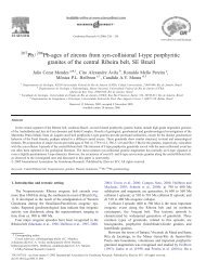
This is an exact solution of a spherically symmetric, non 

asymptotically flat (NAF), static and electrically charged black 

hole, with event horizon r + (r + ≥ 0). The parameters r + and r 0 

(r 0 ≥ 0) are related to the physical mass 2 and the electric 

charge by: 

√ 

(1 − γ) 

(1 + γ) 

M = r + , q = ±r 0 . (11) 

4 

2η 2 

Considering the normal and phantom cases, one gets the 

following interval γ ∈ (−∞, +1). 

2 We use the quasi-local mass. 





Conclusion 

Figure: Penrose diagrams for NAF black holes. 





Conclusion 

The thermodynamics variables 

The Hawking temperature, the entropy and electric potential of 

the black hole are give by 

[ 

g ′ ] 

00 

T = 

4π √ = r γ + 

−g 00 g 11 r = r + 4πr 1+γ , (12) 

0 

S = 1 4 A = 1 ∫ 

√g22 g 33 dθdφ∣ = πr 1+γ 

4 

0 

r 1−γ 

+ , (13) 

r=r+ 

√ 

A 0 = − r + 1 + γ 

, (14) 

2r 0 2η 2 

which satisfies the first law of black hole thermodynamics, 

dM = TdS + η 2 A 0 dq . (15) 





Conclusion 

Also, we obtain the following equations of state 

( ) ( ) 

∂M 

∂M 

= T , = η 2 A 0 . (16) 

∂S 

∂q 

q 

For studying the thermodynamics of a geometric form, it is 

useful to write the temperature, entropy and the electric 

potential in functions of the mass and the electric charge. To do 

this, from (11) we get 

r 0 = q 

√ 

S 

2η 2 

1 + γ , r + = 4M 

1 − γ , (17) 

which, from (12), (13) and (14) provides the temperature, the 

entropy and the electric potential in functions of the mass and 

the electric charge 

T = T 1 M γ q −(1+γ) , T 1 = 2 3γ−5 

2 


π 

[η 2 (1 + γ)] 1+γ 

2 

(1 − γ) γ , (18) 

(19) 




Conclusion 

Also, we obtain the following equations of state 

( ) ( ) 

∂M 

∂M 

= T , = η 2 A 0 . (16) 

∂S 

∂q 

q 

For studying the thermodynamics of a geometric form, it is 

useful to write the temperature, entropy and the electric 

potential in functions of the mass and the electric charge. To do 

this, from (11) we get 

r 0 = q 

√ 

S 

2η 2 

1 + γ , r + = 4M 

1 − γ , (17) 

which, from (12), (13) and (14) provides the temperature, the 

entropy and the electric potential in functions of the mass and 

the electric charge 

T = T 1 M γ q −(1+γ) , T 1 = 2 3γ−5 

2 


π 

[η 2 (1 + γ)] 1+γ 

2 

(1 − γ) γ , (18) 

(19) 




Conclusion 

S = S 1 M 1−γ q 1+γ , S 1 = 

π2 5−3γ 

2 

(1 − γ) γ−1 , (20) 

[η 2 (1 + γ)] 1+γ 

2 

( ) 

M 

1 + γ 

A 0 = −Ā0 

q , Ā0 = η 2 . (21) 

1 − γ 

One can invert (20) for writing the mass in terms of the entropy 

and the electric charge 

( ) 1 

M(S, q) = q − 1+γ 

1−γ 

S 1−γ 

. (22) 

S 1 

Then, one can express the specific heat as 

( ) ( ) 

∂M ∂M 

/ ( ∂ 2 M 

C q = = 

= 

∂T ∂S 

q 

q 

∂S 2 )q 

(1 − γ) 

S . (23) 

γ 





Conclusion 

The usual thermodynamics analysis 

Let us start our study of the thermodynamics of the class of 

NAF black hole solutions of EMD theory, using the analysis of 

the specific heat. The specific heat calculated by the use of the 

mass is directly proportional to the entropy, as shown in (23). 

Then, as we have a single horizon r + , there are no extreme 

case nor phase transition. So, the geometric methods that 

present acceptable results must reproduce the result of the 

specific heat. In general, the thermodynamics system presents 

thermodynamic interaction, since both the specific heat and the 

temperature of the black hole are non null, but do not possess 

the extreme case, nor phase transition. 





Conclusion 

The Weinhold method 

One of the first to formulate a geometric analysis for a 

thermodynamic system was Weinhold. His method, known as 

the Weinhold method , is to define a metric of the 

thermodynamic space of equilibrium states, through the mass 

as thermodynamic potential. This metric is used for the 

calculation of the curvature scalar R W , which determine 

whether the system possesses phase transitions. The 

Weinhold metric is given by 

dl 2 W (M) 

= ∂2 M 

∂S 2 dS2 + 2 ∂2 M 

∂S∂q dSdq + ∂2 M 

∂q 2 dq2 





Conclusion 

= 

γq − 1+γ 

1−γ 

S 2 (1 − γ) 2 ( S 

S 1 

) 1 

1−γ 

dS 2 − 2 

2(1 + γ) 

− 

(1 − γ) 2 q 3−γ 

1−γ 

2 

(1 + γ)q− 1−γ 

S(1 − γ) 2 ( ) 1 

S 1−γ 

dSdq 

S 1 

( ) 1 

S 1−γ 

dq 2 . 

S 1 

(24) 

The curvature scalar of this metric is identically null and this 

shows that the system can not be analysed as having or not 

phase transition. 





Conclusion 

The Ruppeiner method 

Ruppeiner also introduced a metric for defining the geometry of 

the thermodynamic space of the equilibrium states, but in this 

case, with the entropy as a thermodynamic potential. Again, 

this metric provides a curvature scalar R R , which shows if the 

system possesses thermodynamic interaction and phase 

transitions. The Ruppeiner metric is given by 

dl 2 R(S) 

= − ∂2 S 

∂M 2 dM2 − 2 ∂2 S 

∂M∂q dMdq − ∂2 S 

∂q 2 dq2 

= S 2 1 γ(1 − γ)M−1−γ q 1+γ dM 2 − 2S 1 (1 + γ)(1 − γ)M −γ q γ × 

×dMdq − S 1 γ(1 + γ)M 1−γ q −1+γ dq 2 . (25) 

The curvature scalar of this metric is identically null. This 

means that there is no thermodynamic interaction, which does 

not agree with the result obtained by the specific heat. 





Conclusion 

The geometrothermodynamics method 

Hernando Quevedo has improved the following metric for the 

thermodynamic space of the equilibrium states 

( 

dlG(Φ) 2 = E c ∂Φ ) ( 

∂E c η ad δ di ∂ 2 ) 

Φ 

∂E i E b dE a dE b , (26) 

where Φ is the thermodynamics potential and E a are the 

extensive thermodynamics variables. For the thermodynamic 

potential being the entropy (20), the metric (26) has to be given 

by 

( 

dlG(S) 2 = M ∂S 

∂M + q ∂S ) ( 

) 

− ∂2 S 

∂q ∂M 2 dM2 + ∂2 S 

∂q 2 dq2 (27) 

= 2S 2 1 γ(1 − γ)M−2γ q 2(1+γ) dM 2 

+ 2S 2 1 γ(1 + γ)M2(1−γ) q 2γ dq 2 . (28) 

The curvature scalar of this metric is identically zero 





Conclusion 

Making the calculus for the metric (26), using the mass (22) as 

thermodynamic potential, on gets 

dlG(M) 2 = 

(1+γ 

γ2 −2 ( ) 2 

q 

(1−γ) S 1−γ 

dS 2 2γ(1 + γ) 

S 2 (1 − γ) 3 − S 1 (1 − γ) 3 q− 1−γ × 

( ) 2 

S 1−γ 

× dq 2 . 

S 1 

(29) 

The curvature scalar of this metric is also identically zero. Once 

again the incompatibility with the analysis of GTD with that of 

specific heat has been obtained. This was first shown in 

pathological solutions of phantom black holes 3 and next in 

(anti) Reissner-Nordstrom-AdS black holes 4 . 

3 Manuel E. Rodrigues and Zui A.A. Oporto, Phys.Rev. D85 (2012) 104022. 

4 Deborah F. Jardim, Manuel E. Rodrigues and Stephane J. M. Houndjo, 

Eur.Phys.J.Plus 127 (2012) 123. 





Conclusion 

The Liu-Lu-Luo-Shao method 

Recently, Liu-Luo-Lu-Shao, in the same order as Weinhold, has 

formulated a metric of the thermodynamic space of the 

equilibrium states, which provides a curvature scalar that 

determines whether the system possesses phase transitions. 

This metric is a new thermodynamic metric based on the 

Hessian matrix of several free energy, which in the case of the 

Helmholtz free energy, is given by 

dlLLLS(F 2 ) 

= −dTdS + dA 0 dq = − γT ( ) γ 

(1+γ) 

1 

q− (1−γ) S 1−γ 

dS 

2 

S 1 

− 

S(1 − γ) 

q −2 ( ) 1 

1−γ S 1−γ [Ā0 − (1 + γ)T 1 S ] dSdq 

S(1 − γ) S 1 

+ 2Ā0 (3−γ) 

q− (1−γ) 

(1 − γ) 

( S 

S 1 

) 1 

1−γ 

dq 2 . (30) 





Conclusion 

The curvature scalar of this metric is identically null. As we had 

seen, this result also is not in accordance with that of the 

specific heat. An inconsistency with respect to the specific heat 

was shown for the topological case of black hole in 

Horava-Lifshitz gravity 5 . 

5 Qiao-Jun Cao, Yi-Xin Chen and Kai-Nan Shao, Phys.Rev.D 83: 064015 

(2011). 

Manuel E. Rodrigues and Glauber T. Marques Thermodynamics of a class of non-asymptotically flat black h



Conclusion 

The local and global stability 

We now have to study the stability of this thermodynamic 

system. With respect to this, we may split into two parts, the 

local stability and the global one. 

The local stability is easily analysed by the specific heat (23) 

C q = 

(1 − γ) 

S . (31) 

γ 

Here, we see that for the normal case of EMD (η 1 = η 2 = 1), 

the system is always locally stable for 0 < γ < 1, i.e. C q > 0, 

and locally unstable for −1 < γ < 0. But for the phantom case, 

the system is always locally unstable, since γ ∈ (−∞, −1). 





Conclusion 

The local and global stability 

We now have to study the stability of this thermodynamic 

system. With respect to this, we may split into two parts, the 

local stability and the global one. 

The local stability is easily analysed by the specific heat (23) 

C q = 

(1 − γ) 

S . (31) 

γ 

Here, we see that for the normal case of EMD (η 1 = η 2 = 1), 

the system is always locally stable for 0 < γ < 1, i.e. C q > 0, 

and locally unstable for −1 < γ < 0. But for the phantom case, 

the system is always locally unstable, since γ ∈ (−∞, −1). 





Conclusion 

Now we can analyse the global stability of the thermodynamic 

system. First, we define the Gibbs potential in the grand 

canonical ensemble 

G = M − TS − η 2 A 0 q = M(1 − T 1 S 1 + η 2 Ā 0 ) = 

M 

1 − γ . (32) 

So, we see that there is no change of the Gibbs potential, 

unless for the variation of the parameter γ. For the normal 

case, γ ∈ (−1, 1), the potential is always positive and then, the 

system is globally unstable. But the phantom case, 

γ ∈ (−∞, −1), appears as the opposite of the previous one, 

and the system is globally stable. This is not consistent with our 

previous analysis, so that the Gibbs potential, for the grand 

canonical ensemble, does not seem suitable to do this analysis. 





Conclusion 

On the other hand, the analysis made by the Helmholtz free 

energy in the canonical ensemble, shows a good agreement 

with the results already obtained in this work. We define the 

Helmholtz free energy as 

F = M − TS = M(1 − T 1 S 1 ) = − γM 

1 − γ . (33) 

Now the situation seems to have been reversed. In the normal 

case, we have F < 0 for 0 < γ < 1, which leads to a globally 

stable system, such as the local stability made by the specific 

heat. However, the phantom case is always globally unstable. 





Conclusion 

a) We calculated the extensive and intensives variable for this 

thermodynamic system. The first law of thermodynamics is 

also established in (15). 

b) We analysed the thermodynamic system by the geometric 

methods of the geometrothermodynamics, Weinhold, 

Ruppeiner and that of Liu-Lu-Luo-Shao. All analysis by the 

geometric methods provided an identically null curvature scalar 

for the thermodynamic space of the equilibrium states. This is 

incompatible with the analysis made by the usual specific heat, 

which provides an interacting system without extreme case or 






Conclusion 

a) We calculated the extensive and intensives variable for this 

thermodynamic system. The first law of thermodynamics is 

also established in (15). 

b) We analysed the thermodynamic system by the geometric 

methods of the geometrothermodynamics, Weinhold, 

Ruppeiner and that of Liu-Lu-Luo-Shao. All analysis by the 

geometric methods provided an identically null curvature scalar 

for the thermodynamic space of the equilibrium states. This is 

incompatible with the analysis made by the usual specific heat, 

which provides an interacting system without extreme case or 






Conclusion 

c) The local stability analysis done by the specific heat and the 

global stability made by the Helmholtz free energy in the 

canonical ensemble, shows that the normal case is locally and 

globally stable for −1 < λ < 1 (0 < γ < 1). On the other hand, 

for the other intervals of γ, including all phantom cases, the 

system becomes unstable. 

Thank you very much. 

Muito Obrigado. 





Conclusion 

c) The local stability analysis done by the specific heat and the 

global stability made by the Helmholtz free energy in the 

canonical ensemble, shows that the normal case is locally and 

globally stable for −1 < λ < 1 (0 < γ < 1). On the other hand, 

for the other intervals of γ, including all phantom cases, the 

system becomes unstable. 

Thank you very much. 

Muito Obrigado.

Thermodynamics of a class of non-asymptotically flat black holes in ...

You also want an ePaper? Increase the reach of your titles

Delete template?

Save as template?