Knapsack problem, Huffman Code, Single Source Shortest Path ...

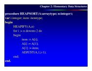
Chapter 4: The Greedy Method
Greedy Technique: Given n inputs, obtain a subset that satisfy
some constraints.
feasible solution: any subset that satisfies all the
constraints.
optimal solution: feasible solution which maximizes
(or minimizes a) given objective function.
there is usually an obvious way to determine a feasible
solution, but not necessarily an optimal solution.
1

Chapter 4: The Greedy Method
The greedy method suggests that one can device an algorithm
which works in stages taking one input at a time.
At any stage, a decision is made whether or not a particular
input is in optimal solution. This is done by considering the
input in an order determined by some selection procedure.
The selection procedure itself is based on some optimization
measure.
Several different optimization measures may be plausible for a
given problem. 2

Chapter 4: The Greedy Method
Global solution: set of items;
procedure Greedy (A:arraytype; n:integer);
{A[1..n] contains n inputs, output available in global “solution”}
var x: item;
begin
solution := ; {initialize the solution to be empty}
for i:= 1 to n do
begin
x := SELECT(A);
if FEASIBLE(solution, x) then
solution := UNION(solution, x);
end {required solution is now available in solution}
end.
3

Chapter 4: The Greedy Method
The function SELECT selects an input from A, removes
it and assign its value to x.
FEASIBLE is a boolean values function which
determines if x can be included in the solution vector.
UNION actually combines x with solution and updates
the objective function.
4

Chapter 4: The Greedy Method
Knapsack problem
Given n objects and a knapsack. Object i has weight w i and
knapsack has capacity M.
If a fraction x i , 0 x i 1, of object i is placed into the
knapsack, then a profit of p i x i is earned.
Problem may be stated as-
Maximize p i x i , 1 i n ........................(1)
Subject to x M , 1 i n ........................(2)
w i i
5

Chapter 4: The Greedy Method
profits and weights are positive numbers
0 x 1, for 1 i n ...........................(3)
i
A feasible solution is any set (x 1 , x 2 , ..., x n ) satisfying
(2) and (3).
An optimal solution is a feasible for which (1) is
maximum.
6

Chapter 4: The Greedy Method
Example: Consider the following instance of the knapsack
problem:
n=3, M=20, (P 1 , P 2 , P 3 ) = (25, 24, 15), (w 1 , w 2 , w 3 ) = (18, 15, 10).
four feasible solutions are:
Sr.No (x 1 , x 2 , x 3 )
w i x i
p i xi
1 (1/2, 1/3, 1/4) 16.5 24.25
2 (1, 2/15, 0) 20 28.2
3 (0, 2/3, 1) 20 31
Maximum 4 (0, profit 1, 1/2) per unit of 20capacity used 31.5
7

Chapter 4: The Greedy Method
Global real P(1:n), W(1:n), X(1:n), M, cu;
procedure GREEDY_KNAPSACK(P, W, X, M, n)
// n objects ordered so that P(i)/W(i) P(i+1)/W(i+1). M is the
knapsack size and X(1:n) is the solution vector.//
var n: integer;
begin
X := 0; //initialize solution to zero//
cu := M; //cu = remaining knapsack capacity//
for i := 1 to n do
begin
if W(i) > cu then exit
X(i) := 1; cu := cu - W(i);
end
if ( i n ) then X(i) := cu/W(i);
end.
8

Chapter 4: The Greedy Method
Huffman code:
What is Morse code
How characters are represented in the memory of the
computer
Which is a fixed length code
A byte is enough to store any number, there are 256 possible
codes, which is more than enough!
9

Chapter 4: The Greedy Method
We need less than that.
Assume the existence of the five letters ‘a’, ‘b’, ‘c’, ‘d’, ‘e’.
Three bits give us 8 possible different sequences.
letter
code
a 000
b 001
c 010
d 011
e 100
Average code length = 3
10

Chapter 4: The Greedy Method
Possibility 1:
Suppose that we know the percentage of occurrence of a
character
‘a’ = 35%, ‘b’ = 20%, ‘c’ = 20%, ‘d’ = 15%, ‘e’ = 10%, then
we can define a variable length code.
letter frequency code
a .35 0
b .20 1
c .20 00
d .15 01
e .10 10
11

Chapter 4: The Greedy Method
Average code length = 1(.35)+1(.20)+2(.20)+2(.15)+1(.10) =
1.35, half that we did with last code. Unfortunately it does not
work. What is 0010
aaba, aae, cba or ce?
Possibility 2:
Each row begins with 11 and 11 will not be used other than to
coding space.
12

Chapter 4: The Greedy Method
Average code length = 3.35
letter frequency code
a .35 110
b .20 111
c .20 1100
d .15 1101
e .10 1110
13

Chapter 4: The Greedy Method
Possibility 3:
Code has a prefix property. “No code be prefix to another”.
letter frequency code
a .35 00
b .20 10
c .20 010
d .15 011
e .10 111
Average code length = 2.45
On these discussions D.A. Huffman proposed minimal length
prefix codes. We begin with forest of trees, correspondence to
single character in the alphabet, weight associated with it. 14

Chapter 4: The Greedy Method
procedure HUFFMAN_CODE
1. repeat
i. find two trees of smallest weight, merge them
together by making them the left and right
children of a new root.
ii. make the weight of the new tree equals to the
sum of the weights of two subtrees
until (the forest consists of a single tree)
2. assign to each left edge a value 0 and each right edge the
value 1.
3. read the codes for the letters by tracking down the tree. 15

Chapter 4: The Greedy Method
letter frequency code
a .35 10
b .20 00
c .20 01
d .15 110
e .10 111
16

Chapter 4: The Greedy Method
a b c d e
.35 .20 .20 .15 .10
17

Chapter 4: The Greedy Method
.25
a b c d e
.35 .20 .20
18

Chapter 4: The Greedy Method
.40
.25
a b c d e
.35
19

Chapter 4: The Greedy Method
.40
.60
b
c
a
d
e
20

Chapter 4: The Greedy Method
b c a
d
e
21

Chapter 4: The Greedy Method
0
1
0
1
0
1
b c a
0
1
d
Average Code length = 2.25
e
One more Ex.?
22

Chapter 4: The Greedy Method
SINGLE SOURCE SHORTEST PATH PROBLEM
In general shortest path problems are concerned with finding
paths between vertices.
Some characteristics which may help in finding the exact
problem is-
1. Graph is finite or infinite
2. Graph is directed or undirected
23

Chapter 4: The Greedy Method
3. Edges are all of length 1, or all lengths are non
negative, or negative lengths are allowed.
4. We may be interested in shortest path from a given
vertex to another, or, from a given vertex to all other
vertices, or, from each vertex to all the other vertices.
Is there a path from A to B?
Is there any other path from A to B which is shortest
path?
length of the path = sum of weights of the edges on that path.
24

Chapter 4: The Greedy Method
We assume that starting vertex is the source and the last vertex
is the destination, directed graph G = (V, E) a weighting
function c(e) for the edges of G and a source vertex v 0 .
20
45
50 10
V 0
V 1 V 4
10 15
20 35 30
V 2 V
15
3
V
3
5
25
Path Length
V 0 V 2 10
V 0 V 2 V 3 25
V 0 V 2 V 3 V 1 45
V 0 V 4 45

Chapter 4: The Greedy Method
In order to generate the shortest path we need to be able to
determine
1. The next vertex to which the shortest path must be
generated.
2. Shortest path to this vertex.
Let S denotes the set of all vertices (including v 0 to which the
path has already been generated).
for w not in S, let DIST(w) be the length of the shortest path
starting from v 0 going through only those vertices which are in
S and ending at w, we observe-
26

Chapter 4: The Greedy Method
1. If next shortest path is to u, then path begins at v 0
end to u, going through only those vertices which
are in S. {Assume that there is a vertex w not in S,
path v 0 to u contains a path from v 0 to w which is
of length less than the v 0 to u path, which
contradicts the existence of such w.}
2.The destination of the next path generated must be
that vertex u which has the minimum distance,
DIST(u), among all vertices not in S.
27

Chapter 4: The Greedy Method
3. Having selected such u from (2) above, and generated
the shortest path v 0 to u, u becomes the member of S.
length of this path is DIST(u) + c(u,w).
The algorithms is known as Dijkstra’s Algorithm
28

Chapter 4: The Greedy Method
3. Having selected such u from (2) above, and generated
the shortest path v 0 to u, u becomes the member of S.
length of this path is DIST(u) + c(u,w).
Procedure SHORTEST-PATHS(v, COST, DIST, n)
//DIST(j), 1 j n is set to the length of the Shortest path
from v to j.//
//DIST(v) is set to 0//
var boolean S(1:n); real COST(1:n, 1:n), DIST(1:n)
integer u, v, n, num, i, w;
begin
for i := 1 to n do //initialize set S to empty//
29

Chapter 4: The Greedy Method
begin
S[i] := 0; DIST(i) := COST[v,i];
end
S[v] := 1; DIST[v] := 0; //put the vertex v in set S//
for num := 2 to n-1 do //determine n-1 paths from
vertex v//
begin
choose u such that DIST[u] = min{DIST(w)}
S[w] := 0;
S[u] := 1; //put vertex u in set S//
for all w with S[w] = 0 do //update distances//
DIST[w] := min{DIST(w), DIST(u) +COST(u,w)}
end
end. 30

Chapter 4: The Greedy Method
3250
San 800
Francisco
300
2
Los
Angeles
1
Denver
3
1200
2450
Chicago
1000
1650
Miami
1400
New
3350 Orleans
7
1700 8
1000
4
1000
1250
1500
Boston
6
5
New York
900
250
1150
31

Chapter 4: The Greedy Method
End of Chapter 4
32