- Page 1 and 2: The Computable Differential Equatio
- Page 3 and 4: Contents 1 Classifying The Problem
- Page 5 and 6: CONTENTS v Timeline on Computable D
- Page 7 and 8: Chapter 1 Classifying The Problem 1
- Page 9 and 10: CHAPTER 1. CLASSIFYING THE PROBLEM
- Page 11 and 12: CHAPTER 1. CLASSIFYING THE PROBLEM
- Page 13 and 14: CHAPTER 1. CLASSIFYING THE PROBLEM
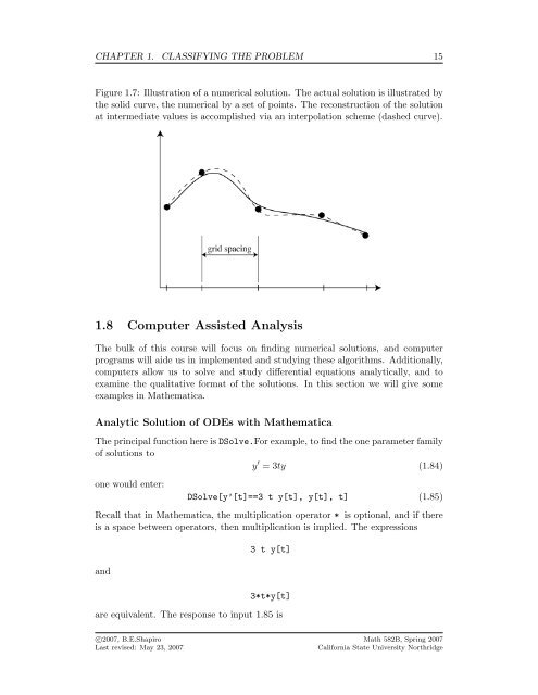
- Page 15 and 16: CHAPTER 1. CLASSIFYING THE PROBLEM
- Page 17 and 18: CHAPTER 1. CLASSIFYING THE PROBLEM
- Page 19: CHAPTER 1. CLASSIFYING THE PROBLEM
- Page 23 and 24: CHAPTER 1. CLASSIFYING THE PROBLEM
- Page 25 and 26: CHAPTER 1. CLASSIFYING THE PROBLEM
- Page 27 and 28: CHAPTER 1. CLASSIFYING THE PROBLEM
- Page 29 and 30: CHAPTER 1. CLASSIFYING THE PROBLEM
- Page 31 and 32: Chapter 2 Successive Approximations
- Page 33 and 34: CHAPTER 2. SUCCESSIVE APPROXIMATION
- Page 35 and 36: CHAPTER 2. SUCCESSIVE APPROXIMATION
- Page 37 and 38: CHAPTER 2. SUCCESSIVE APPROXIMATION
- Page 39 and 40: CHAPTER 2. SUCCESSIVE APPROXIMATION
- Page 41 and 42: CHAPTER 2. SUCCESSIVE APPROXIMATION
- Page 43 and 44: CHAPTER 2. SUCCESSIVE APPROXIMATION
- Page 45 and 46: CHAPTER 2. SUCCESSIVE APPROXIMATION
- Page 47 and 48: CHAPTER 2. SUCCESSIVE APPROXIMATION
- Page 49 and 50: Chapter 3 Approximate Solutions 3.1
- Page 51 and 52: CHAPTER 3. APPROXIMATE SOLUTIONS 45
- Page 53 and 54: CHAPTER 3. APPROXIMATE SOLUTIONS 47
- Page 55 and 56: CHAPTER 3. APPROXIMATE SOLUTIONS 49
- Page 57 and 58: CHAPTER 3. APPROXIMATE SOLUTIONS 51
- Page 59 and 60: CHAPTER 3. APPROXIMATE SOLUTIONS 53
- Page 61 and 62: CHAPTER 3. APPROXIMATE SOLUTIONS 55
- Page 63 and 64: CHAPTER 3. APPROXIMATE SOLUTIONS 57
- Page 65 and 66: CHAPTER 3. APPROXIMATE SOLUTIONS 59
- Page 67 and 68: CHAPTER 3. APPROXIMATE SOLUTIONS 61
- Page 69 and 70: CHAPTER 3. APPROXIMATE SOLUTIONS 63
- Page 71 and 72:
CHAPTER 3. APPROXIMATE SOLUTIONS 65
- Page 73 and 74:
CHAPTER 3. APPROXIMATE SOLUTIONS 67
- Page 75 and 76:
Chapter 4 Improving on Euler’s Me
- Page 77 and 78:
CHAPTER 4. IMPROVING ON EULER’S M
- Page 79 and 80:
CHAPTER 4. IMPROVING ON EULER’S M
- Page 81 and 82:
CHAPTER 4. IMPROVING ON EULER’S M
- Page 83 and 84:
CHAPTER 4. IMPROVING ON EULER’S M
- Page 85 and 86:
CHAPTER 4. IMPROVING ON EULER’S M
- Page 87 and 88:
CHAPTER 4. IMPROVING ON EULER’S M
- Page 89 and 90:
CHAPTER 4. IMPROVING ON EULER’S M
- Page 91 and 92:
CHAPTER 4. IMPROVING ON EULER’S M
- Page 93 and 94:
CHAPTER 4. IMPROVING ON EULER’S M
- Page 95 and 96:
Chapter 5 Runge-Kutta Methods 5.1 T
- Page 97 and 98:
CHAPTER 5. RUNGE-KUTTA METHODS 91 w
- Page 99 and 100:
CHAPTER 5. RUNGE-KUTTA METHODS 93 w
- Page 101 and 102:
CHAPTER 5. RUNGE-KUTTA METHODS 95 5
- Page 103 and 104:
CHAPTER 5. RUNGE-KUTTA METHODS 97 F
- Page 105 and 106:
CHAPTER 5. RUNGE-KUTTA METHODS 99 T
- Page 107 and 108:
CHAPTER 5. RUNGE-KUTTA METHODS 101
- Page 109 and 110:
CHAPTER 5. RUNGE-KUTTA METHODS 103
- Page 111 and 112:
CHAPTER 5. RUNGE-KUTTA METHODS 105
- Page 113 and 114:
CHAPTER 5. RUNGE-KUTTA METHODS 107
- Page 115 and 116:
CHAPTER 5. RUNGE-KUTTA METHODS 109
- Page 117 and 118:
CHAPTER 5. RUNGE-KUTTA METHODS 111
- Page 119 and 120:
CHAPTER 5. RUNGE-KUTTA METHODS 113
- Page 121 and 122:
CHAPTER 5. RUNGE-KUTTA METHODS 115
- Page 123 and 124:
Chapter 6 Linear Multistep Methods
- Page 125 and 126:
CHAPTER 6. LINEAR MULTISTEP METHODS
- Page 127 and 128:
CHAPTER 6. LINEAR MULTISTEP METHODS
- Page 129 and 130:
CHAPTER 6. LINEAR MULTISTEP METHODS
- Page 131 and 132:
CHAPTER 6. LINEAR MULTISTEP METHODS
- Page 133 and 134:
CHAPTER 6. LINEAR MULTISTEP METHODS
- Page 135 and 136:
CHAPTER 6. LINEAR MULTISTEP METHODS
- Page 137 and 138:
CHAPTER 6. LINEAR MULTISTEP METHODS
- Page 139 and 140:
CHAPTER 6. LINEAR MULTISTEP METHODS
- Page 141 and 142:
Chapter 7 Delay Differential Equati
- Page 143 and 144:
CHAPTER 7. DELAY DIFFERENTIAL EQUAT
- Page 145 and 146:
CHAPTER 7. DELAY DIFFERENTIAL EQUAT
- Page 147 and 148:
CHAPTER 7. DELAY DIFFERENTIAL EQUAT
- Page 149 and 150:
CHAPTER 7. DELAY DIFFERENTIAL EQUAT
- Page 151 and 152:
CHAPTER 7. DELAY DIFFERENTIAL EQUAT
- Page 153 and 154:
CHAPTER 7. DELAY DIFFERENTIAL EQUAT
- Page 155 and 156:
CHAPTER 7. DELAY DIFFERENTIAL EQUAT
- Page 157 and 158:
CHAPTER 7. DELAY DIFFERENTIAL EQUAT
- Page 159 and 160:
Chapter 8 Boundary Value Problems 8
- Page 161 and 162:
CHAPTER 8. BOUNDARY VALUE PROBLEMS
- Page 163 and 164:
CHAPTER 8. BOUNDARY VALUE PROBLEMS
- Page 165 and 166:
CHAPTER 8. BOUNDARY VALUE PROBLEMS
- Page 167 and 168:
CHAPTER 8. BOUNDARY VALUE PROBLEMS
- Page 169 and 170:
CHAPTER 8. BOUNDARY VALUE PROBLEMS
- Page 171 and 172:
CHAPTER 8. BOUNDARY VALUE PROBLEMS
- Page 173 and 174:
Chapter 9 Differential Algebraic Eq
- Page 175 and 176:
CHAPTER 9. DIFFERENTIAL ALGEBRAIC E
- Page 177 and 178:
CHAPTER 9. DIFFERENTIAL ALGEBRAIC E
- Page 179 and 180:
CHAPTER 9. DIFFERENTIAL ALGEBRAIC E
- Page 181 and 182:
CHAPTER 9. DIFFERENTIAL ALGEBRAIC E
- Page 183 and 184:
CHAPTER 9. DIFFERENTIAL ALGEBRAIC E
- Page 185 and 186:
CHAPTER 9. DIFFERENTIAL ALGEBRAIC E
- Page 187 and 188:
CHAPTER 9. DIFFERENTIAL ALGEBRAIC E
- Page 189 and 190:
CHAPTER 9. DIFFERENTIAL ALGEBRAIC E
- Page 191 and 192:
CHAPTER 9. DIFFERENTIAL ALGEBRAIC E
- Page 193 and 194:
CHAPTER 9. DIFFERENTIAL ALGEBRAIC E
- Page 195 and 196:
CHAPTER 9. DIFFERENTIAL ALGEBRAIC E
- Page 197 and 198:
CHAPTER 9. DIFFERENTIAL ALGEBRAIC E
- Page 199 and 200:
Chapter 10 Appendix on Analytic Met
- Page 201 and 202:
CHAPTER 10. APPENDIX ON ANALYTIC ME
- Page 203 and 204:
CHAPTER 10. APPENDIX ON ANALYTIC ME
- Page 205 and 206:
Bibliography [1] Ascher, Uri M., Ma