The Computable Differential Equation Lecture ... - Bruce E. Shapiro

CHAPTER 8. BOUNDARY VALUE PROBLEMS 157
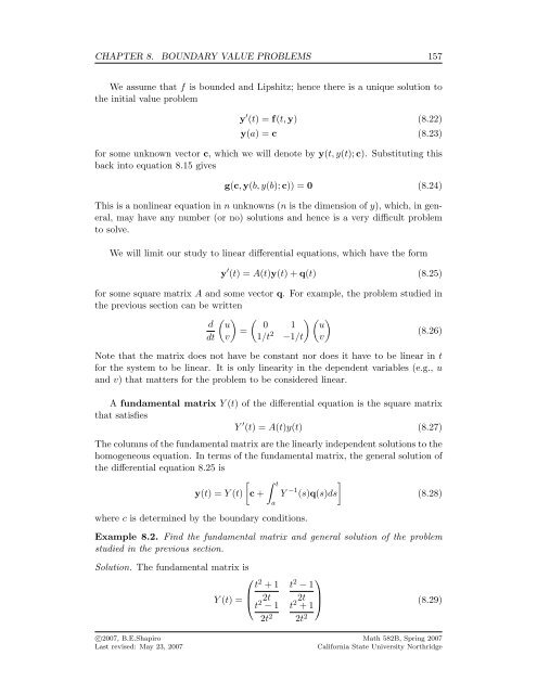
We assume that f is bounded and Lipshitz; hence there is a unique solution to
the initial value problem
y ′ (t) = f(t, y) (8.22)
y(a) = c (8.23)
for some unknown vector c, which we will denote by y(t, y(t); c). Substituting this
back into equation 8.15 gives
g(c, y(b, y(b); c)) = 0 (8.24)
This is a nonlinear equation in n unknowns (n is the dimension of y), which, in general,
may have any number (or no) solutions and hence is a very difficult problem
to solve.
We will limit our study to linear differential equations, which have the form
y ′ (t) = A(t)y(t) + q(t) (8.25)
for some square matrix A and some vector q. For example, the problem studied in
the previous section can be written
( ) ( ( )
d u 0 1 u
=
dt v 1/t −1/t) 2 (8.26)
v
Note that the matrix does not have be constant nor does it have to be linear in t
for the system to be linear. It is only linearity in the dependent variables (e.g., u
and v) that matters for the problem to be considered linear.
A fundamental matrix Y (t) of the differential equation is the square matrix
that satisfies
Y ′ (t) = A(t)y(t) (8.27)
The columns of the fundamental matrix are the linearly independent solutions to the
homogeneous equation. In terms of the fundamental matrix, the general solution of
the differential equation 8.25 is
y(t) = Y (t)
[
c +
∫ t
where c is determined by the boundary conditions.
a
]
Y −1 (s)q(s)ds
(8.28)
Example 8.2. Find the fundamental matrix and general solution of the problem
studied in the previous section.
Solution. The fundamental matrix is
⎛
t 2 + 1
⎜
Y (t) = ⎝ 2t
t 2 − 1
2t
t 2 − 1 t 2 + 1
2t 2 2t 2
⎞
⎟
⎠ (8.29)
c○2007, B.E.Shapiro
Last revised: May 23, 2007
Math 582B, Spring 2007
California State University Northridge