The Computable Differential Equation Lecture ... - Bruce E. Shapiro
The Computable Differential Equation Lecture ... - Bruce E. Shapiro The Computable Differential Equation Lecture ... - Bruce E. Shapiro
8 CHAPTER 1. CLASSIFYING THE PROBLEM Theorem 1.6. Suppose that |∂f/∂y| is bounded by K on a set D. Then f(t, y) ∈ L(y, K)(D). Proof. The result follows immediately from the mean value theorem. Let (t, y 1 ), (t, y 2 ) ∈ D. Then there is some number c between y 1 and y 2 such that Hence f is Lipshitz in y on D. |f(t, y 1 ) − f(t, y 2 )| = |f y (c)||y 1 − y 2 | < K|y 1 − y 2 | (1.29) Example 1.3. Show that a unique solution exists to the initial value problem y ′ = sin(ty), y(0) = 0.5 (1.30) Solution. We have f(t, y) = sin(ty), hence f y = t cos(ty). Thus |f y | ≤ |t| which is bounded for any finite range of t. Let R be a bounded, convex set enclosing (0, 0.5), and let K = 1 + sup |t| (1.31) t∈R Since R is bounded we know that the supremum exists. By adding 1 we ensure that we have a number that is strictly larger than the maximum value of |t|. Then K is a Lipshitz constant for f and hence a unique solution exists in some neighborhood N of (0, 5). See figure 1.5. Figure 1.5: A solution exists in some neighborhood N of (0, 0.5). See Example 1.3 Example 1.4. Analyze the uniqueness of solutions to y ′ = √ 4 − y 2 (1.32) y(0) = 2 (1.33) Math 582B, Spring 2007 California State University Northridge c○2007, B.E.Shapiro Last revised: May 23, 2007
CHAPTER 1. CLASSIFYING THE PROBLEM 9 Solution. Finding a “solution” is easy enough. We can separate the variables and integrate. It is easily verified (by direct substitution) that ( y = 2 sin t + π ) (1.34) 2 satisfies both the differential equation and the initial condition, hence it is a solution. It is also easily verified that y = 2 is a solution, as are functions of the form ⎧ ⎪⎨ 2 sin ( t + π ) 2 t < 0 y = 2 0 ≤ t ≤ φ ⎪⎩ 2 sin ( t + π 2 − φ) t > φ (1.35) for any positive real number φ. See Figure 1.6. Figure 1.6: There are several solutions to y ′ = √ 4 − y 2 that pass through the point (0, 2). See Example 1.4 Since the solution is not unique, any condition that guarantees existence must be violated. We have two such conditions: the boundedness of the partial derivative, and the Lipshitz condition. The first implies the second, and the second implies uniqueness. By ∂f ∂y = −y √ 4 − y 2 (1.36) which is unbounded at y = 2. So the first condition is violated. Of course, a violation of the condition does not ensure non-uniqueness, all it tells us is that uniqueness is not ensured. What about the Lipshitz condition? Suppose that the function f(x) = √ (4−y 2 ) is Lipshitz with Lipshitz constant K > 0 on some domain D. Then for any y 1 , y 2 in c○2007, B.E.Shapiro Last revised: May 23, 2007 Math 582B, Spring 2007 California State University Northridge
- Page 1 and 2: The Computable Differential Equatio
- Page 3 and 4: Contents 1 Classifying The Problem
- Page 5 and 6: CONTENTS v Timeline on Computable D
- Page 7 and 8: Chapter 1 Classifying The Problem 1
- Page 9 and 10: CHAPTER 1. CLASSIFYING THE PROBLEM
- Page 11 and 12: CHAPTER 1. CLASSIFYING THE PROBLEM
- Page 13: CHAPTER 1. CLASSIFYING THE PROBLEM
- Page 17 and 18: CHAPTER 1. CLASSIFYING THE PROBLEM
- Page 19 and 20: CHAPTER 1. CLASSIFYING THE PROBLEM
- Page 21 and 22: CHAPTER 1. CLASSIFYING THE PROBLEM
- Page 23 and 24: CHAPTER 1. CLASSIFYING THE PROBLEM
- Page 25 and 26: CHAPTER 1. CLASSIFYING THE PROBLEM
- Page 27 and 28: CHAPTER 1. CLASSIFYING THE PROBLEM
- Page 29 and 30: CHAPTER 1. CLASSIFYING THE PROBLEM
- Page 31 and 32: Chapter 2 Successive Approximations
- Page 33 and 34: CHAPTER 2. SUCCESSIVE APPROXIMATION
- Page 35 and 36: CHAPTER 2. SUCCESSIVE APPROXIMATION
- Page 37 and 38: CHAPTER 2. SUCCESSIVE APPROXIMATION
- Page 39 and 40: CHAPTER 2. SUCCESSIVE APPROXIMATION
- Page 41 and 42: CHAPTER 2. SUCCESSIVE APPROXIMATION
- Page 43 and 44: CHAPTER 2. SUCCESSIVE APPROXIMATION
- Page 45 and 46: CHAPTER 2. SUCCESSIVE APPROXIMATION
- Page 47 and 48: CHAPTER 2. SUCCESSIVE APPROXIMATION
- Page 49 and 50: Chapter 3 Approximate Solutions 3.1
- Page 51 and 52: CHAPTER 3. APPROXIMATE SOLUTIONS 45
- Page 53 and 54: CHAPTER 3. APPROXIMATE SOLUTIONS 47
- Page 55 and 56: CHAPTER 3. APPROXIMATE SOLUTIONS 49
- Page 57 and 58: CHAPTER 3. APPROXIMATE SOLUTIONS 51
- Page 59 and 60: CHAPTER 3. APPROXIMATE SOLUTIONS 53
- Page 61 and 62: CHAPTER 3. APPROXIMATE SOLUTIONS 55
- Page 63 and 64: CHAPTER 3. APPROXIMATE SOLUTIONS 57
8 CHAPTER 1. CLASSIFYING THE PROBLEM<br />
<strong>The</strong>orem 1.6. Suppose that |∂f/∂y| is bounded by K on a set D. <strong>The</strong>n f(t, y) ∈<br />
L(y, K)(D).<br />
Proof. <strong>The</strong> result follows immediately from the mean value theorem. Let (t, y 1 ), (t, y 2 ) ∈<br />
D. <strong>The</strong>n there is some number c between y 1 and y 2 such that<br />
Hence f is Lipshitz in y on D.<br />
|f(t, y 1 ) − f(t, y 2 )| = |f y (c)||y 1 − y 2 | < K|y 1 − y 2 | (1.29)<br />
Example 1.3. Show that a unique solution exists to the initial value problem<br />
y ′ = sin(ty), y(0) = 0.5 (1.30)<br />
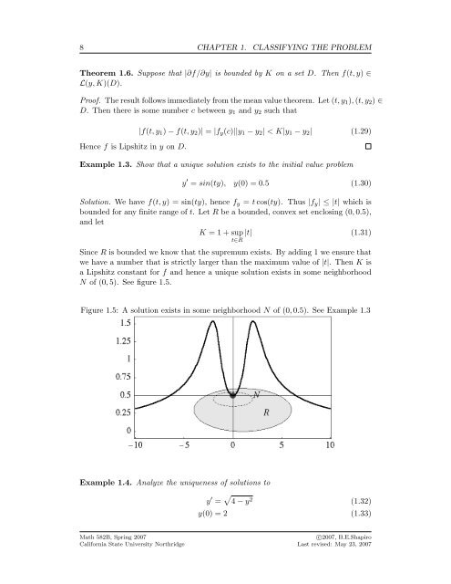
Solution. We have f(t, y) = sin(ty), hence f y = t cos(ty). Thus |f y | ≤ |t| which is<br />
bounded for any finite range of t. Let R be a bounded, convex set enclosing (0, 0.5),<br />
and let<br />
K = 1 + sup |t| (1.31)<br />
t∈R<br />
Since R is bounded we know that the supremum exists. By adding 1 we ensure that<br />
we have a number that is strictly larger than the maximum value of |t|. <strong>The</strong>n K is<br />
a Lipshitz constant for f and hence a unique solution exists in some neighborhood<br />
N of (0, 5). See figure 1.5.<br />
Figure 1.5: A solution exists in some neighborhood N of (0, 0.5). See Example 1.3<br />
Example 1.4. Analyze the uniqueness of solutions to<br />
y ′ = √ 4 − y 2 (1.32)<br />
y(0) = 2 (1.33)<br />
Math 582B, Spring 2007<br />
California State University Northridge<br />
c○2007, B.E.<strong>Shapiro</strong><br />
Last revised: May 23, 2007


