The Computable Differential Equation Lecture ... - Bruce E. Shapiro

94 CHAPTER 5. RUNGE-KUTTA METHODS
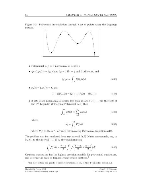
Figure 5.2: Polynomial interpolation through a set of points using the Lagrange
method.
• Polynomial p i (t) is a polynomial of degree i;
• 〈p i (t), p j (t)〉 = δ ij where δ ij = 1 if i = j and 0 otherwise, and
〈f, g〉 =
• p 0 (t) = 1, p 1 (t) = t, and
∫ 1
−1
f(t)g(t)dt (5.36)
(i + 1)P i+1 (t) = (2i + 1)tP i (t) − iP i−1 (t) (5.37)
• If q(t) is any polynomial of degree less than 2n and t 1 , t 2 , . . . are the roots of
the n th Legendre Orthogonal Polynomal p n (t) then
∫ 1
−1
q(t)dt =
n∑
w i q(t i ) (5.38)
i=1
where
w i =
∫ 1
−1
P (t)dt (5.39)
where P (t) is the n th Lagrange Interpolating Polynomial (equation 5.32).
The problem can be translated from any interval [a, b] (which corresponds, say, to
[t 0 , t]), to the interval [−1, 1] by the transformation
∫ b
a
f(t)dt = b − a
2
∫ 1
−1
f
( b − a
2 t + a + b )
dt (5.40)
2
Gaussian quadrature has the highest precision possible for polynomial quadrature,
and it forms the basis of Implicit Runge Kutta methods. 1
1 For more details and proofs of these observations see [6], section 4.7 and [13], section 3.1.
Math 582B, Spring 2007
California State University Northridge
c○2007, B.E.Shapiro
Last revised: May 23, 2007