Lesson 14 Synthetic Division and Horner's Method - Bruce E. Shapiro

Lesson 14
Synthetic Division and Horner’s
Method
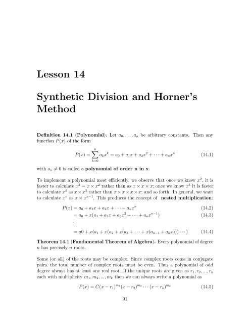
Definition 14.1 (Polynomial). Let a 0 , . . . , a n be arbitrary constants. Then any
function P (x) of the form
P (x) =
n∑
a k x k = a 0 + a 1 x + a 2 x 2 + · · · + a n x n (14.1)
k=0
with a n ≠ 0 is called a polynomial of order n in x.
To implement a polynomial most efficiently, we observe that once we know x 2 , it is
faster to calculate x 3 = x × x 2 rather than as x × x × x; once we know x 3 it is faster
to calculate x 4 as x × x 3 rather than x × x × x × x; and so forth. In general, we want
to calculate x n as x × x n−1 . This produces the concept of nested multiplication:
P (x) = a 0 + a 1 x + a 2 x + · · · + a n x n (14.2)
.
= a 0 + x(a 1 + a 2 x + a 3 x 2 + · · · + a n x n−1 ) (14.3)
= a0 + x(a 1 + x(a 2 + x(a 3 + · · · + x(a n−1 + a n x))) · · · ) (14.4)
Theorem 14.1 (Fundamental Theorem of Algebra). Every polynomial of degree
n has precisely n roots.
Some (or all) of the roots may be complex. Since complex roots come in conjugate
pairs, the total number of complex roots must be even. Thus a polynomial of odd
degree always has at least one real root. If the unique roots are given as r 1 , r 2 , ..., r k
each with multiplicity m 1 , m 2 , ..., m k then we can always write a polynomial as
P (x) = C(x − r 1 ) m 1
(x − r 2 ) m2 · · · (x − r k ) m k
(14.5)
91

92 LESSON 14. SYNTHETIC DIVISION AND HORNER’S METHOD
Descarte proposed in 1637 that one could imagine that there were n roots to a polynomial.
Albert Girard (1629) proposed that an n th order polynomial has n roots but
that they may exist in a field larger than the complex numbers. The first published
proof of the fundamental theorem of algebra was by DAlembert in 1746, but his proof
was based on an earlier theorem that itself used the theorem, and hence is unsatisfactory.
At about the same time Euler proved it for polynomials with real coefficients up
to 6th. Between 1799 (in his doctoral dissertation) and 1816 Gauss published three
different proofs for polynomials with with real coefficients, and in 1849 he proved the
general case for polynomials with complex coefficients.
Theorem 14.2. If two polynomials of degree n agree at n + 1 unique points, then
they must be identical. More precisely: If P (x) and Q(x) are two polynomials of the
same degree n that agree at at least n + 1 distinct points, i.e, if there exist unique
numbers x 1 , ..., x n+1 such that P (x k ) = Q(x k ) then P (x) = Q(x) for all x.
For example, if two lines are equal at two points, they are identical; if two parabolas
match at three points, they are identical; and so on.
Theorem 14.3 (Horner’s Method for Synthetic Division). Let P (x) be any
polynomial of degree n, given by
P (x) = a 0 + a 1 x + a 2 x + · · · + a n x n (14.6)
Then for any number x 0 there exists another polynomial Q(x) of degree n − 1, given
by
Q(x) = b 1 + b 2 x + b 3 x 2 + · · · + b n x n−1 (14.7)
such that
where b n = a n ,
P (x) = (x − x 0 )Q(x) + b 0 (14.8)
b k = a k + b k+1 x 0 (14.9)
for k = n − 1, n − 2, ..., 0, for k = n − 1, n − 2, . . . , 0 Furthermore, b 0 = P (x 0 ) and
Proof. Suppose that
P ′ (x 0 ) = Q(x 0 ) (14.10)
Q(x) = b n x n−1 + b n−1 x n−2 + · · · + b 3 x 2 + b 2 x + b 1 (14.11)
for some undetermined numbers b 1 , . . . , b n . Then we ask what conditions will ensure
that
P (x) = (x − x 0 )Q(x) + b 0 (14.12)
Math 481A
California State University Northridge
2008, B.E.Shapiro
Last revised: November 16, 2011

LESSON 14. SYNTHETIC DIVISION AND HORNER’S METHOD 93
Multiplying things out,
(x − x 0 )Q(x) + b 0 = b 0 +
(x − x 0 )(b n x n−1 + b n−1 x n−2 + · · · + b 3 x 2 + b 2 x + b 1 ) (14.13)
= b 0 + x(b n x n−1 + b n−1 x n−2 + · · · + b 3 x 2 + b 2 x + b 1 )
− x 0 (b n x n−1 + b n−1 x n−2 + · · · + b 3 x 2 + b 2 x + b 1 ) (14.14)
= b n x n + b n−1 x n−1 + b n−2 x n−2 + · · · + b 2 x 2 + b 1 x
− b n x 0 x n−1 − x 0 b n−1 x n−2 − · · · − x 0 b 3 x 2
− x 0 b 2 x − x 0 b 1 + b 0 (14.15)
= b n x n + (b n−1 − b n x 0 )x n−1 +
(b n−2 − x 0 b n−1 )x n−2 + · · · + (14.16)
(b 2 − x 0 b 3 )x 2 + (b 1 − x 0 b 2 )x + (b 0 − x 0 b 1 ) (14.17)
We want this to be equal to
P (x) = a 0 + a 1 x + a 2 x + · · · + a n x n (14.18)
Equating coefficients of like powers of x gives us
a n = b n (14.19)
a n−1 = b n−1 − b n x 0 (14.20)
a n−2 = b n−2 − b n−1 x 0 (14.21)
.
a 0 = b 0 − x 0 b 1 (14.22)
Rearranging,
b n = a n (14.23)
b n−1 = a n−1 + b n x 0 (14.24)
b n−2 = a n−2 + b n−1 x 0 (14.25)
.
b 0 = a 0 + b 1 x 0 (14.26)
This proves equation 14.9.
Next, to see that b 0 = P (x 0 ) we observe that
P (0) = (x 0 − x 0 )Q(x 0 ) + b 0 = b 0 (14.27)
Furthermore, differentiating P (x) = (x − x 0 )Q(x) + b 0 gives
P ′ (x) = (x − x 0 )Q ′ (x) + Q(x) (14.28)
2008, B.E.Shapiro
Last revised: November 16, 2011
Math 481A
California State University Northridge

94 LESSON 14. SYNTHETIC DIVISION AND HORNER’S METHOD
hence
which gives us equation 14.10.
P ′ (x 0 ) = Q(x 0 ) (14.29)
The following gives a recapitulation of the algorithm for Horner’s method to calculate
the numbers P (x 0 ) and P ′ (x 0 ) for a polynomial.
Algorithm Horner
Input a 0 , . . . , a n , x 0 ;
Set y = a n ; (y will give the b n for P )
Set z = a n ; (z gives the b n−1 for Q)
For j = n − 1, n − 2, . . . , 1,
y = x 0 y + a j ; (this gives b j for P (x 0 ))
z = x 0 z + y; (this gives b j−1 for the calculation of Q(x 0 ) )
End For;
y = x 0 y + a 0 ; (this gives b 0 )
Return y (which is P (x 0 )) and z (which is P ′ (x 0 ) = Q(x 0 ))
We can make two interesting observations about Horner’s method. First, it has the
same number of multiplications as nested multiplication, making it at least as efficient
as that algorithm. Secondly, it gives us a number for both P (x 0 ) and P ′ (x 0 ) for no
extra cost. This becomes useful in operations where both numbers are needed, such
as in the calculation of Newton’s method (for the roots of a polynomial).
Algorithm Newton’s Method with Horner
Input a 0 , . . . , a n , x 0 , tolerance ɛ;
(p 0 , p ′ 0) = Horner(a 0 , . . . , a n , x 0 )
p = x 0
δ = p 0 /p ′ 0
While |δ| > ɛ,
p = p − δ
(p 0 , p ′ 0) = Horner(a 0 , . . . , a n , p)
δ = p 0 /p ′ 0
End While
Return p
Let x 0 be a root of P . Then we know that there exists a second polynomial Q(x) such
that P (x) = (x − x 0 )Q(x) + P (x 0 ) = (x − x 0 )Q(x). So if P has any other roots that
are different from x 0 then they are also roots of Q. Hence if we repeat the process on
Q iteratively we will find all the subsequent roots of P . Unfortunately this leads to
round-off error that can be avoided by using a different algorithm that we will discuss
subsequently.
Math 481A
California State University Northridge
2008, B.E.Shapiro
Last revised: November 16, 2011

LESSON 14. SYNTHETIC DIVISION AND HORNER’S METHOD 95
Example 14.1. Find P (1) and P ′ (1) for P (x) = x 3 −2x 2 −5 using Horner’s method.
Solution. We have a 0 = −5, a 1 = 0, a 2 = −2, and a 3 = 1, and also x 0 = 1. Then If
we set z = a 3 = 1,
b 3 = a 3 = 1 (14.30)
b 2 = a 2 + b 3 x 0 = −2 + (1)(1) = −1 (14.31)
b 1 = a 1 + b 2 x 0 = 0 + (−1)(1) = −1 (14.32)
b 0 = a 0 + b 1 x 0 = −5 + (−1)(1) = −6 (14.33)
Hence P (1) = −6. Using the same algorithm for Q we have
Hence Q(1) = P ′ (1) = c 0 = −1.
c 2 = b 3 = 1 (14.34)
c 1 = b 2 + c 2 x 0 = (−1) + (1)(1) = 0 (14.35)
c 0 = b 1 + c 1 x 0 = (−1) + (0)(1) = −1 (14.36)
Horner’s method is also fairly easy to implement in Mathematica. We can take
advantage of the fact that a list may have an arbitrary number of elements, so we
don’t even need to know the order of the polynomial:
Horner[A_?ListQ, x0_] := Module[{z, y, a},
a = A;
y = z = Last[a];
a = Most[a];
While[Length[a] > 1,
y = x0*y + Last[a];
z = x0*z + y;
a = Most[a];
];
y = x0*y + Last[a];
Print["P(x)=" A.("x"^Range[0, Length[A] - 1])];
Print["P(", x0, ")=", y, "\n", "P’(", x0, ")=", z];
Return[{y, z}]
]
2008, B.E.Shapiro
Last revised: November 16, 2011
Math 481A
California State University Northridge

96 LESSON 14. SYNTHETIC DIVISION AND HORNER’S METHOD
Math 481A
California State University Northridge
2008, B.E.Shapiro
Last revised: November 16, 2011