Multivariate Calculus - Bruce E. Shapiro
Multivariate Calculus - Bruce E. Shapiro Multivariate Calculus - Bruce E. Shapiro
176 LECTURE 22. LINE INTEGRALS and breaking the path itself up into points Let us define the differential vector and the differential time element Then in the limit as dt i → 0, we have r(t 1 ), r(t 2 ), ..., r(t n ) (22.2) dr i = r(t i+1 ) − t i (22.3) dt i = t i+1 − t i (22.4) lim dr i = r ′ (t i )dt = v(t i )dt (22.5) dt i →0 Now suppose that the curve is embedded in some vector field F(r). Then at any Figure 22.2: Partitioning of an oriented curve into small segments that approximate the tangent vectors. point r along the curve we can calculate the dot product r(t) · F(r(t)) This product is a measure of how much alignment there is between the motion along the curve and the direction of the vector field. The dot product is maximized when the angle between the two vectors is zero, and we are moving “with the flow” of the field. If we are moving completely in the opposite direction, the dot product is negative, and if we move in a direction perpendicularly to the vector field than the dot product is zero, as there is no motion with with or against the flow. We define the line integral of f along C as the Riemann Sum ∫ n∑ F · dr = lim dr i · F(r i ) (22.6) dr i →0 or equivalently ∫ C C F · dr = ∫ b a i=1 [ dr dt · F(r(t)) ] dt (22.7) Revised December 6, 2006. Math 250, Fall 2006
LECTURE 22. LINE INTEGRALS 177 Example 22.1 Find the line integral of the vector field F(r(t)) = (2x, 3y, 0) over the path ABC as illustrated in figure 22.3 Figure 22.3: The oriented curve ABC referenced in example 22.1 Solution. We can parameterize the curve as { (t, 2, 0) 0 ≤ t ≤ 10 r(t) = (10, t − 8, 0) 10 ≤ t ≤ 18 (22.8) Based on this parameterization, we can write equations for the individual coordinates x(t) and y(t) { t 0 ≤ t ≤ 10 x(t) = (22.9) 10 10 ≤ t ≤ 18 { 2 0 ≤ t ≤ 10 y(t) = (22.10) t − 8 10 ≤ t ≤ 18 and for the velocity Therefore r ′ (t) = { (1, 0, 0) 0 ≤ t ≤ 10 (0, 1, 0) 10 ≤ t ≤ 18 { F · r ′ (2x, 3y, 0) · (1, 0, 0) 0 ≤ t ≤ 10 = (2x, 3y, 0) · (0, 1, 0) 10 ≤ t ≤ 18 { 2x 0 ≤ t ≤ 10 = 3y 10 ≤ t ≤ 18 { 2t 0 ≤ t ≤ 10 = 3(t − 8) 10 ≤ t ≤ 18 (22.11) (22.12) (22.13) (22.14) Math 250, Fall 2006 Revised December 6, 2006.
- Page 137 and 138: LECTURE 15. CONSTRAINED OPTIMIZATIO
- Page 139 and 140: Lecture 16 Double Integrals over Re
- Page 141 and 142: LECTURE 16. DOUBLE INTEGRALS OVER R
- Page 143 and 144: LECTURE 16. DOUBLE INTEGRALS OVER R
- Page 145 and 146: LECTURE 16. DOUBLE INTEGRALS OVER R
- Page 147 and 148: Lecture 17 Double Integrals over Ge
- Page 149 and 150: LECTURE 17. DOUBLE INTEGRALS OVER G
- Page 151 and 152: LECTURE 17. DOUBLE INTEGRALS OVER G
- Page 153 and 154: LECTURE 17. DOUBLE INTEGRALS OVER G
- Page 155 and 156: LECTURE 17. DOUBLE INTEGRALS OVER G
- Page 157 and 158: Lecture 18 Double Integrals in Pola
- Page 159 and 160: LECTURE 18. DOUBLE INTEGRALS IN POL
- Page 161 and 162: LECTURE 18. DOUBLE INTEGRALS IN POL
- Page 163 and 164: LECTURE 18. DOUBLE INTEGRALS IN POL
- Page 165 and 166: LECTURE 18. DOUBLE INTEGRALS IN POL
- Page 167 and 168: Lecture 19 Surface Area with Double
- Page 169 and 170: LECTURE 19. SURFACE AREA WITH DOUBL
- Page 171 and 172: LECTURE 19. SURFACE AREA WITH DOUBL
- Page 173 and 174: Lecture 20 Triple Integrals Triple
- Page 175 and 176: LECTURE 20. TRIPLE INTEGRALS 163 Fi
- Page 177 and 178: LECTURE 20. TRIPLE INTEGRALS 165 so
- Page 179 and 180: LECTURE 20. TRIPLE INTEGRALS 167 Tr
- Page 181 and 182: Lecture 21 Vector Fields Definition
- Page 183 and 184: LECTURE 21. VECTOR FIELDS 171 Defin
- Page 185 and 186: LECTURE 21. VECTOR FIELDS 173 Examp
- Page 187: Lecture 22 Line Integrals Suppose t
- Page 191 and 192: LECTURE 22. LINE INTEGRALS 179 ener
- Page 193 and 194: LECTURE 22. LINE INTEGRALS 181 The
- Page 195 and 196: LECTURE 22. LINE INTEGRALS 183 so t
- Page 197 and 198: LECTURE 22. LINE INTEGRALS 185 wher
- Page 199 and 200: LECTURE 22. LINE INTEGRALS 187 The
- Page 201 and 202: LECTURE 22. LINE INTEGRALS 189 The
- Page 203 and 204: Lecture 23 Green’s Theorem Theore
- Page 205 and 206: LECTURE 23. GREEN’S THEOREM 193 T
- Page 207 and 208: Lecture 24 Flux Integrals & Gauss
- Page 209 and 210: LECTURE 24. FLUX INTEGRALS & GAUSS
- Page 211 and 212: LECTURE 24. FLUX INTEGRALS & GAUSS
- Page 213 and 214: Lecture 25 Stokes’ Theorem We hav
- Page 215 and 216: LECTURE 25. STOKES’ THEOREM 203 S
176 LECTURE 22. LINE INTEGRALS<br />
and breaking the path itself up into points<br />
Let us define the differential vector<br />
and the differential time element<br />
Then in the limit as dt i → 0, we have<br />
r(t 1 ), r(t 2 ), ..., r(t n ) (22.2)<br />
dr i = r(t i+1 ) − t i (22.3)<br />
dt i = t i+1 − t i (22.4)<br />
lim dr i = r ′ (t i )dt = v(t i )dt (22.5)<br />
dt i →0<br />
Now suppose that the curve is embedded in some vector field F(r). Then at any<br />
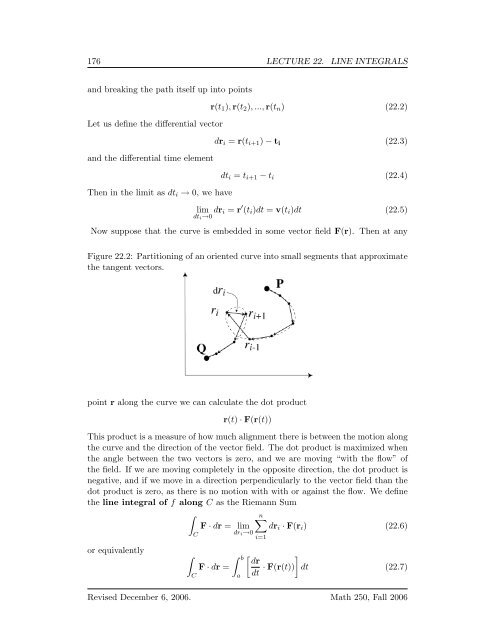
Figure 22.2: Partitioning of an oriented curve into small segments that approximate<br />
the tangent vectors.<br />
point r along the curve we can calculate the dot product<br />
r(t) · F(r(t))<br />
This product is a measure of how much alignment there is between the motion along<br />
the curve and the direction of the vector field. The dot product is maximized when<br />
the angle between the two vectors is zero, and we are moving “with the flow” of<br />
the field. If we are moving completely in the opposite direction, the dot product is<br />
negative, and if we move in a direction perpendicularly to the vector field than the<br />
dot product is zero, as there is no motion with with or against the flow. We define<br />
the line integral of f along C as the Riemann Sum<br />
∫<br />
n∑<br />
F · dr = lim dr i · F(r i ) (22.6)<br />
dr i →0<br />
or equivalently<br />
∫<br />
C<br />
C<br />
F · dr =<br />
∫ b<br />
a<br />
i=1<br />
[ dr<br />
dt · F(r(t)) ]<br />
dt (22.7)<br />
Revised December 6, 2006. Math 250, Fall 2006


