Review of Partial Derivatives - Bruce E. Shapiro
Review of Partial Derivatives - Bruce E. Shapiro
Review of Partial Derivatives - Bruce E. Shapiro

You also want an ePaper? Increase the reach of your titles
YUMPU automatically turns print PDFs into web optimized ePapers that Google loves.
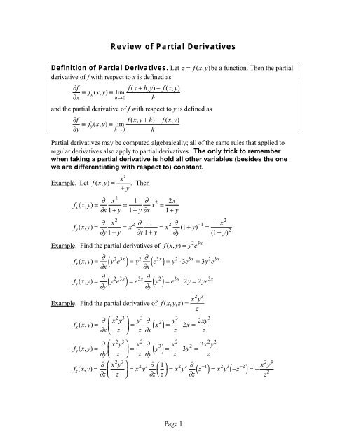
<strong>Review</strong> <strong>of</strong> <strong>Partial</strong> <strong>Derivatives</strong><br />
Definition <strong>of</strong> <strong>Partial</strong> <strong>Derivatives</strong>. Let z = f( x, y)be a function. Then the partial<br />
derivative <strong>of</strong> f with respect to x is defined as<br />
∂f<br />
∂ ≡ ≡ f x+ h y − f x y<br />
fx( x, y) lim ( , ) ( , )<br />
x<br />
h→0<br />
h<br />
and the partial derivative <strong>of</strong> f with respect to y is defined as<br />
∂f<br />
∂ ≡ ≡ f x y+ k − f x y<br />
fy( x, y) lim ( , ) ( , )<br />
y<br />
k→0<br />
k<br />
<strong>Partial</strong> derivatives may be computed algebraically; all <strong>of</strong> the same rules that applied to<br />
regular derivatives also apply to partial derivatives. The only trick to remember<br />
when taking a partial derivative is hold all other variables (besides the one<br />
we are differentiating with respect to) constant.<br />
2<br />
x<br />
Example. Let f( x, y)= . Then<br />
1 + y<br />
2<br />
x<br />
fx ( x , y )= ∂<br />
x + y = 1 ∂<br />
+ y x x 2 2<br />
=<br />
∂ 1 1 ∂ 1 +<br />
xy<br />
2<br />
x<br />
x<br />
f y ( x , y ) ∂<br />
= x x y<br />
y + y<br />
= 2 ∂ 1<br />
y + y<br />
= 2 ∂<br />
y<br />
( + ) −1<br />
1 = − ∂ 1 ∂ 1 ∂<br />
( 1 + y )<br />
Example. Find the partial derivatives <strong>of</strong> f( x, y)= y 2 e 3x<br />
∂<br />
f x y<br />
x ye y ∂<br />
x( , )= ( )= (<br />
x e )= y ⋅ 3 e = 3<br />
∂<br />
∂<br />
y e<br />
∂<br />
f x y<br />
y ye 2 3x e 3x ∂<br />
y<br />
y y 2 e 3x y ye 3x<br />
( , )= ( )= ( )= ⋅ 2 = 2<br />
∂<br />
∂<br />
2 3x 2 3x 2 3x 2 3x<br />
Example. Find the partial derivative <strong>of</strong> f( x, y, z)=<br />
fx ( x , y )=<br />
∂ ⎛<br />
∂x<br />
⎜<br />
⎝<br />
fy ( x , y )= ∂ ⎛<br />
∂y<br />
⎜<br />
⎝<br />
fz ( x , y )= ∂ ⎛<br />
∂z<br />
⎜<br />
⎝<br />
2 3 3<br />
x y<br />
z<br />
x y<br />
z<br />
2 3<br />
x y<br />
z<br />
3 3<br />
⎞ y<br />
z x x y xy<br />
⎟ x<br />
⎠<br />
= ∂ 2<br />
2<br />
( )= ⋅ 2 =<br />
∂ z z<br />
2 3 2<br />
2 3<br />
x y<br />
z<br />
2<br />
2 2<br />
⎞ xz y y x x y<br />
⎟ y<br />
⎠<br />
= ∂ 3<br />
2 3<br />
( )= ⋅ 3 =<br />
∂ z z<br />
⎞<br />
x y x y<br />
z z z z x y z x y<br />
⎟<br />
⎠<br />
= 2 3 ∂ ⎛ 1⎞<br />
⎝ ⎠ = 2 3 ∂ −1 2 3 −2<br />
( )= ( − )=−<br />
2<br />
∂<br />
∂<br />
z<br />
2<br />
2<br />
2 3<br />
Page 1
Second Order <strong>Partial</strong> <strong>Derivatives</strong><br />
We define higher order partial derivatives in much the same way as we did in single-variable<br />
calculus.<br />
f f<br />
fxx<br />
= ∂ 2<br />
= ∂ ⎛ ∂ ⎞<br />
2 ⎜ ⎟<br />
∂x<br />
∂x<br />
⎝ ∂x⎠<br />
2<br />
f f<br />
fyy<br />
= ∂ = ∂ ⎛ ∂ ⎞<br />
2 ⎜ ⎟<br />
∂y<br />
∂y<br />
⎝ ∂y⎠<br />
With partial derivatives, we can also combine the variables, so there are more derivatives at<br />
each order. For example, we can differentiate f x with respect to y and we can differentiate<br />
f y with respect to x:<br />
f<br />
xy<br />
2<br />
f f<br />
= ∂ ⎛ ∂ ⎞<br />
⎜ ⎟ = ∂ ∂x<br />
⎝ ∂y⎠<br />
∂∂ xy<br />
2<br />
f f<br />
fyx<br />
= ∂ ⎛ ∂ ⎞<br />
⎜ ⎟ = ∂ ∂y<br />
⎝ ∂x⎠<br />
∂∂ yx<br />
We can, <strong>of</strong> course, combine higher order derivatives in any order we like. For example:<br />
f f<br />
fxxyx = ∂ 4<br />
∂ ∂ ∂<br />
∂x ∂x ∂y<br />
∂ x<br />
= ∂<br />
2<br />
∂ xyx ∂ ∂<br />
There are not as many partials as you might think, however, because <strong>of</strong> the following<br />
theorem:<br />
f f<br />
The order <strong>of</strong> the partials can be reversed: fxy<br />
= ∂ 2<br />
fyx<br />
∂∂ xy<br />
= ∂ 2<br />
∂∂ yx<br />
=<br />
Example. Find all the second-order partial derivatives <strong>of</strong> f( x, y)= xy 2 + 3 x 2 e y and show<br />
that fxy<br />
= fyx<br />
by taking partials in both orders.<br />
2 y<br />
y<br />
y<br />
y<br />
fx<br />
= y + xe ⇒ fxx<br />
= e fyx<br />
= ∂ 2<br />
6 6 , ( y + 6xe )= 2y+<br />
6xe<br />
∂y 2 y<br />
2 y<br />
y<br />
y<br />
fy<br />
= xy+ x e ⇒ fyy<br />
= x+ x e fxy<br />
= ∂ 2<br />
2 3 2 3 , ( 2xy + 3x e )= 2y + 6xe = f<br />
∂x<br />
Example. Repeat the above example for f( x, y)=<br />
xe y<br />
f = e ⇒ f = 0,<br />
f = e<br />
x<br />
y<br />
xx<br />
f = xe ⇒ f = xe , f = e = f<br />
y<br />
y<br />
yy<br />
y<br />
yx<br />
xy<br />
y<br />
y<br />
yx<br />
yx<br />
Page 2
Chain Rule<br />
If zt () = f( xt (), yt ()) then the chain rule is<br />
dz f dx f dy<br />
= ∂ + ∂ dt ∂x<br />
dt ∂y<br />
dt<br />
In general, if z is a function <strong>of</strong> any number <strong>of</strong> variables xt ( ), yt ( ), zt ( ), wt ( ), ... , each <strong>of</strong><br />
which can be expressed as a function <strong>of</strong> only t (and not <strong>of</strong> any other parameter),<br />
d<br />
dt f x y z w f dx f dy f dz f dw<br />
( , , , ,... )= ∂ + ∂ + ∂ + ∂ +<br />
∂x<br />
dt ∂y<br />
dt ∂z<br />
dt ∂w<br />
dt<br />
...<br />
Example. Suppose f( x, y) = xsin<br />
y, where x = t<br />
2 and y = 2t<br />
+ 1. Then by the chain rule<br />
we have<br />
′ = ∂ f dx<br />
+ ∂ f dy<br />
f () t<br />
∂x<br />
dt ∂y<br />
dt<br />
= ∂ ∂ ( ) ( )+ ∂ x x sin y d dt t 2<br />
∂ y ( x sin y) d dt<br />
( 2t<br />
+ 1 )<br />
= ( sin y)( 2t)+ ( xcos<br />
y)( 2)<br />
= 2tsin( 2t + 1)+ 2t 2<br />
cos( 2t<br />
+ 1)<br />
Page 3
Vector Products<br />
There are two types <strong>of</strong> products between vectors, one <strong>of</strong> which produces a vector and the<br />
other produces a scalar<br />
• The dot product v r ⋅w<br />
r ⎯→⎯<br />
scalar<br />
• The cross product v r × w r ⎯→⎯<br />
vector<br />
The Dot Product is defined geometrically<br />
r r<br />
v⋅ w = v wcosθ<br />
where q is the angle between the two vectors as shown in the<br />
figure. Algebraically, if<br />
r r r r r r r r<br />
v = iv1+ jv2 + kv3 and w = iw1+ jw2 + kw3<br />
r r r r<br />
Then v⋅ w = w⋅ v = v1w1+ v2w2 + v3w3<br />
Example. Suppose that r r r r<br />
u = 3i + 4 j + 5 k and r r r r<br />
v = 7i + 8j + 9k<br />
Then u r ⋅ v<br />
r = ( 3)( 7) + ( 4)( 8) + ( 5)( 9)<br />
= 21 + 32 + 45 = 98<br />
Properties <strong>of</strong> the dot product<br />
r r r r<br />
1. v⋅ w = w⋅v<br />
r r r r r r<br />
2. v⋅ ( aw) = ( av) ⋅ w = a( v⋅w)<br />
3. ( v r + u r ) ⋅ w r = v r ⋅ w r + u r ⋅w<br />
r<br />
r<br />
4. v and ware r perpendicular only if v r ⋅ w<br />
r = 0.<br />
The Cross Product<br />
The cross product is a product between vectors that results in a vector. It is defined as a<br />
vector with the following properties:<br />
• Its length is equal to v r × w r = v r w<br />
r sinθ<br />
• direction is perpendicular to the plane that contains v and w<br />
• Its orientation (up vs. down) is according to the right hand rule<br />
Right-Hand Rule: Place u r and v r so that their tails coincide and curl the fingers <strong>of</strong> your right<br />
hand from through the angle from u r to v r . Your thumb is pointing in the direction <strong>of</strong> u<br />
r × v<br />
r<br />
The cross product gives the area <strong>of</strong> the parallelogram formed by the two vectors:<br />
θ<br />
θ<br />
w|sinθ<br />
v|<br />
Page 4
We can also calculate the cross product algebraically from the components <strong>of</strong> the individual<br />
vectors if we use determinants.<br />
r r r<br />
i j k<br />
r r<br />
r r r<br />
v w v v v i v 2 v 3<br />
j v 1 v 3<br />
k v 1 v 3<br />
× = 1 2 3 = − +<br />
w2 w3<br />
w1 w3<br />
w1 w3<br />
w1 w2 w3<br />
r r r<br />
= i( v w −v w )− j( v w −v w )+ k( v w −v w )<br />
2 3 3 2 1 3 3 1 1 2 2 1<br />
Determinant <strong>of</strong> a Matrix<br />
⎛<br />
det a b ⎞ a b<br />
⎜ ⎟ ≡ ≡ ad −bc<br />
⎝ c d⎠<br />
c d<br />
⎛ a b c⎞<br />
a b c<br />
det⎜d e f⎟<br />
d e f a e f b d f c d e<br />
⎜ ⎟ = = h i<br />
− g i<br />
+ g h<br />
⎝ g h i⎠<br />
g h i<br />
= a( ei − fh) −b( di − fg) + c( dh −eg)<br />
Properties <strong>of</strong> the Cross Product<br />
(1) w r × v r = − v r × w<br />
r<br />
r r r r r r<br />
(2) ( av)× w = a( v × w)= v ×( aw)<br />
(3) u r × ( v r + w r )= u r × v r + u r × w<br />
r<br />
(4) u<br />
r × v<br />
r = 0 if and only if the vectors are parallel (assuming that r r r<br />
uv , ≠ 0)<br />
(5) i r × r j = k r , r j × k r = i r , k r × i r =<br />
r<br />
j (cyclic cross products)<br />
(6) r j × i r = − k r , k r × r j = − i r , i r × k = −<br />
r<br />
j (acyclic cross products)<br />
(7) v<br />
r × v<br />
r = 0<br />
Vector Operators: Gradient, Divergence and Curl<br />
The gradient <strong>of</strong> a function <strong>of</strong> three variables is the vector<br />
r f f<br />
grad f ≡∇f( x, y, z)<br />
≡i<br />
∂ j k<br />
f ∂ x<br />
+ r ∂ ∂ y<br />
+ r ∂ ∂z<br />
We can think <strong>of</strong> the gradient symbol ∇ as a operator that behaves exactly like a vector with<br />
the exception <strong>of</strong> the fact that it operates on the single item immediately to its right.<br />
In this sense, we can think <strong>of</strong> ∇ as vector version <strong>of</strong> ∂ ∂x .<br />
Specifically, ∇ represents the “vector”<br />
r r ∂ r r<br />
∇=<br />
∂ + ∂<br />
∂ + ∂<br />
i j k<br />
x y ∂ z<br />
Page 5
Example. f xe y 2<br />
+<br />
=<br />
z<br />
Then<br />
r r r r r<br />
∇ =∇ ⎛ 2 ⎞<br />
⎝ ⎠ = ⎛ ∂<br />
∂ + ∂<br />
∂ + ∂ ⎞<br />
⎜<br />
⎟ ⎛ 2<br />
f xe i j k xe<br />
⎝ x y ∂ z ⎠⎝<br />
y + z y + z<br />
r ∂ ⎛ ⎞ r r<br />
=<br />
∂ ⎝ ⎠ + ∂ ⎛ ⎞<br />
∂ ⎝ ⎠ + ∂ ⎛<br />
i<br />
x xe 2 j y xe 2 k ∂z ⎝<br />
xe 2<br />
r r r<br />
y<br />
2<br />
+ z y<br />
2<br />
+ z y<br />
2<br />
+ z<br />
= i e + j 2xye + kxe<br />
y + z y + z y + z<br />
Since we are treating ∇ “like a vector,” we can subject to all <strong>of</strong> the usual vector operations,<br />
such as dot product and cross product. We will define the following operations using ∇<br />
Operation Name <strong>of</strong> Operator Input Output<br />
∇ gradient scalar vector<br />
∇⋅ divergence (dot product) vector scalar<br />
read as “del dot ...”<br />
∇× curl (cross product) vector vector<br />
read as “del cross ...”<br />
∇⋅∇ or ∇ 2 Laplacian scalar scalar<br />
read as “del squared ...”<br />
Both the divergence and curl operate on vector functions. A vector function is a function<br />
r r r r<br />
Fxyz ( , , ) = iF( xyz , , ) + jF( xyz , , ) + kF( xyz , , )<br />
1 2 3<br />
where the functions F1, F2, F3<br />
are all real valued functions.<br />
Example <strong>of</strong> a Vector Function. r r 2<br />
Fxyz ( , , )= xi+ yx+<br />
zj r ek<br />
x r<br />
⎞<br />
⎠<br />
( ) +<br />
The Divergence Operator is defined as “del dot a vector function”,<br />
div r r r ⎛ r ∂<br />
F =∇⋅ F = i<br />
r j k r iF r r jF kF<br />
r<br />
∂ x<br />
+ ∂<br />
∂ y<br />
+ ∂ ⎞<br />
⎜<br />
⎟ ⋅ z<br />
( 1+ 2 + 3)<br />
⎝<br />
∂ ⎠<br />
F F F<br />
= ∂ 1<br />
∂ x<br />
+ ∂ 2<br />
∂ y<br />
+ ∂ 3<br />
∂z<br />
Example. Find the divergence <strong>of</strong> r r 2<br />
Fxyz ( , , )= xi+ yx+<br />
zj r ek<br />
x r<br />
⎞<br />
⎠<br />
( ) +<br />
( )<br />
r r ⎛ r ∂ r r r r r<br />
∇⋅ =<br />
∂ + ∂<br />
∂ + ∂ ⎞<br />
2<br />
x<br />
F ⎜i<br />
j k ⎟ ⋅ xi + ( y x + z) j + e k<br />
⎝ x y ∂ z ⎠<br />
= ∂ x<br />
∂ + ∂ 2<br />
( + )+ ∂ = + + = +<br />
x ∂y y x z x<br />
e 1 2xy 0 1 2xy<br />
∂z Page 6
The Curl Operator is defined as “del cross f”<br />
curl r r r ⎛ r ∂<br />
F =∇× F = i<br />
r j k r iF r r jF kF<br />
r<br />
∂ x<br />
+ ∂<br />
∂ y<br />
+ ∂ ⎞<br />
⎜<br />
⎟ × z<br />
( 1+ 2 + 3)<br />
⎝<br />
∂ ⎠<br />
r r r<br />
i j k<br />
r F F r F F r F<br />
= ∂ ∂ ∂<br />
i<br />
j<br />
k<br />
∂x ∂y ∂ z<br />
= ⎛ ∂<br />
∂y<br />
− ∂ ⎞ ⎛ ∂<br />
⎜ ⎟ +<br />
⎝ ∂z<br />
⎠ ∂z<br />
− ∂ ⎞ ⎛ ∂<br />
⎜ ⎟ +<br />
⎝ ∂x<br />
⎠<br />
⎜<br />
⎝ ∂x<br />
F F F<br />
1 2 3<br />
Example. Suppose F r e y r y<br />
= 2 i + 2 xye 2r<br />
j + k<br />
r<br />
r r r<br />
i j k<br />
r r<br />
∇× = ∂ ∂ ∂<br />
F<br />
∂x ∂y ∂z<br />
y<br />
2<br />
y<br />
2<br />
e 2xye<br />
1<br />
− ∂ F ⎞<br />
⎟<br />
∂y<br />
⎠<br />
3 2 1 3 2 1<br />
r⎛<br />
∂<br />
r r<br />
= − ∂ ⎞ ∂<br />
⎜<br />
⎟ + − ∂ ⎛<br />
⎛<br />
⎞ ∂<br />
⎜<br />
⎟ +<br />
− ∂ y<br />
() 1<br />
y<br />
2<br />
i<br />
xye j<br />
⎝ ∂y<br />
∂z<br />
⎠ ⎝ ∂z e y<br />
2 () 1<br />
y<br />
2 e<br />
[ 2 ]<br />
k [ 2xye<br />
]<br />
∂x<br />
⎠ ⎜<br />
⎝<br />
∂x<br />
∂y<br />
r r r<br />
= i( 0−0)+ j( 0−0)+ ⎛ y y<br />
k 2ye 2 −2ye<br />
2 ⎞<br />
⎝<br />
⎠ = 0<br />
The Laplacian Operator is the dot product <strong>of</strong> ∇with itself, or the divergence <strong>of</strong> the<br />
gradient. It is sometimes read as “del squared”.<br />
∇<br />
2 r r<br />
f( x, y, z) =∇⋅ ∇f( x, y, z)<br />
( )<br />
⎛ r ∂<br />
=<br />
∂ + r ∂<br />
∂ +<br />
r ∂ ⎞ ⎡⎛<br />
r ∂<br />
⎜<br />
⎟ ⋅<br />
⎝<br />
∂ ⎠ ∂ + r ∂<br />
∂ +<br />
r ∂ ⎞ ⎤<br />
i j k ⎢⎜i<br />
j k ⎟ f ⎥<br />
x y z ⎣⎝<br />
x y ∂ z ⎠ ⎦<br />
⎛ r ∂<br />
=<br />
∂ + r ∂<br />
∂ +<br />
r ∂ ⎞ ⎛ r∂f<br />
⎜i<br />
j k ⎟ ⋅ i<br />
⎝<br />
∂ ⎠ ∂ + r<br />
j<br />
∂ f<br />
x y z x ∂ +<br />
r ∂ ⎞<br />
⎜<br />
k<br />
f ⎟<br />
⎝ y ∂z⎠<br />
2<br />
= ∂ f<br />
+ ∂ f<br />
+ ∂ f<br />
2 2 2<br />
∂x<br />
∂y<br />
∂z<br />
The Laplacian operates on a scalar and its output is a scalar.<br />
2<br />
2<br />
2<br />
⎞<br />
⎟<br />
⎠<br />
Page 7
Polar Coordinates<br />
In polar coordinates, instead <strong>of</strong> using the distances x and y from the origin to locate a point,<br />
we use a single distance r and an orientation angle with respect to the x-axis.<br />
x=rcosθ<br />
r<br />
y=rsinθ<br />
θ<br />
The two coordinate systems are related to each other as follows:<br />
x = rcosθ<br />
r = x<br />
2<br />
+ y<br />
2<br />
y = rsinθ<br />
y<br />
θ = arctan<br />
x<br />
We can also define unit vectors and r θ at any given point in space; they can be related to<br />
the cartesian unit vectors i r and r j from the following geometry.<br />
r<br />
j<br />
r<br />
θ<br />
θ<br />
θ<br />
r<br />
r<br />
i<br />
P<br />
θ<br />
Since all the vectors shown are unit vectors, we observe that:<br />
x component <strong>of</strong> ˆr is cosθ ;<br />
y component <strong>of</strong> ˆr is sinθ ;<br />
x component <strong>of</strong> ˆθ is −sinθ<br />
y component <strong>of</strong> ˆθ is cosθ<br />
Page 8
Therefore<br />
rˆ = cosθi ˆ + sinθj<br />
ˆ<br />
θˆ =− sinθi<br />
ˆ + cosθj<br />
ˆ<br />
Exercise: Find expressions for î and ĵ in terms <strong>of</strong> ˆr and ˆθ .<br />
Solution. Multiply the first expression by sinθ and the second expression by cosθ<br />
ˆsin sin cos ˆ 2<br />
r θ = θ θi + sin θjˆ<br />
θˆ cos θ cos θ sin θiˆ 2<br />
=− + cos θjˆ<br />
Adding the two expressions,<br />
ˆsin ˆ cos sin<br />
2 ˆ 2<br />
r θ + θ θ = θj + cos θjˆ = jˆ<br />
which gives an expression for ĵ in terms <strong>of</strong> ˆr and ˆθ .<br />
To get a similar expressionf or î , multiply the expression for ˆr by cosθ and the<br />
expression for ˆθ by sinθ ,<br />
2<br />
rˆ cosθ = cos θiˆ + cosθsinθj<br />
ˆ<br />
ˆsin sin<br />
2<br />
θ θ =− θiˆ + cosθsinθj<br />
ˆ<br />
Subtract the bottom expression from the top,<br />
ˆ cos ˆsin cos<br />
2 ˆ 2<br />
r θ − θ θ = θi + sin θiˆ = iˆ<br />
Summarizing the conversion expressions, we have<br />
r r<br />
i = rˆ cosθ −θˆsin<br />
θ r = cosθi + sinθj<br />
and r r r<br />
jˆ = rˆsinθ + θˆ cos θ θ =− sinθi<br />
+ cosθj<br />
Example. Find an expression for the vector field F r = 3xiˆ+<br />
4x 2 yjˆ in polar coordinates.<br />
Solution.<br />
r<br />
F = 3xiˆ<br />
2<br />
+ 4x yjˆ<br />
= 3( rcos θ)(ˆ rcosθ − θˆsin θ ) + 4 ( r cos θ ) ( r sin θ )(ˆ r cos θ + θˆsin θ )<br />
2 3 3 3 2 2<br />
= 3rcos θrˆ − 3rcosθsinθθ ˆ + 4r cos θsinθrˆ + 4r<br />
cos θsin θθˆ<br />
2 3 3<br />
3 2 2<br />
= ( 3rcos θ + 4r cos θsin θ)ˆ r + ( 4r<br />
cos θsin θ − 3rcosθsin θ) θ ˆ<br />
2 2 2<br />
= rcos θ( 3+ 4r cosθsin θ)ˆ r + rcosθsin θ( 4r<br />
cosθsin θ −3) θ ˆ<br />
Exercise: Recall that the gradient in two dimensions in cartesian coordinates is<br />
∇ = ∂ f<br />
f x y i<br />
∂ + ∂ f<br />
( , ) ˆ jˆ . Find an expression for the gradient in polar coordinates, i .e., find<br />
x ∂y<br />
the functions g and h so that ∇ f(, r θ ) = rg ˆ (, r θ ) + θ ˆ h (, r θ ).<br />
Hint: you must use the chain<br />
rule and the expressions for transformation <strong>of</strong> coordinates.<br />
2<br />
Page 9