Lecture Notes in Differential Equations - Bruce E. Shapiro
Lecture Notes in Differential Equations - Bruce E. Shapiro Lecture Notes in Differential Equations - Bruce E. Shapiro
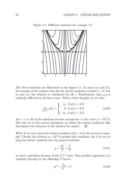
34 LESSON 4. LINEAR EQUATIONS Figure 4.1: Different solutions for example 4.6. 2 1 0 1 2 2 1 0 1 2 The three solutions are illustrated in the figure 4.1. In cases (a) and (b), the domain of the solution that fits the initial condition excludes t = 0; but in case (c), the solution is continuous for all t. Furthermore, lim t→0 y is radically different in all three cases. With a little thought we see that ⎧ ⎪⎨ ∞, if y(1) > 2/3 lim y(t) = 0, if y(1) = 2/3 t→0 + ⎪ ⎩ −∞, if y(1) < 2/3 (4.80) As t → ∞ all of the solutions become asymptotic to the curve y = 2t 2 /3. The side on of the curved asymptote on which the initial conditions falls determines the behavior of the solution for small t. What if we were given the initial condition y(0) = 0 in the previous example? Clearly the solution y = 2t 2 /3 satisfies this condition, but if we try to plug the initial condition into the general solution y = 2t2 3 + C t 4 (4.81) we have a problem because of the C/t 4 term. One possible approach is to multiply through by the offending t 4 factor: yt 4 = 2 3 t6 + C (4.82)
35 Substituting y = t = 0 in this immediately yields C = 0. This problem is a direct consequence of the fact that we divided our equation through by t 4 previously to get an express solution for y(t) (see the transition from equation 4.72 to equation 4.73): this division is only allowed when t ≠ 0. Example 4.7. Solve the initial value problem dy dt − 2ty = √ 2 ⎫ ⎬ π ⎭ y(0) = 0 (4.83) Since p(t) = −2t, an integrating factor is (∫ ) µ = exp −2tdt = e −t2 (4.84) Following our usual procedure we get d ( ye −t2) = √ 2 e −t2 (4.85) dt π If we try to solve the indefinite integral we end up with ye −t2 = √ 2 ∫ e −t2 dt + C (4.86) π Unfortunately, there is no exact solution for the indefinite integral on the right. Instead we introduce a new concept, of finding a definite integral. We will use as our lower limit of integration the initial conditions, which means t = 0; and as our upper limit of integration, some unknown variable u. Then ∫ u Then we have 0 d ( ye −t2) dt = dt ∫ u ( ye −t2) ( − ye −t2) = 2 ∫ u √ t=0 t=u π 0 2 √ π e −t2 dt (4.87) Using the initial condition y(0) = 0, the left hand side becomes 0 e −t2 dt (4.88) y(u)e −(u)2 − y(0)e −(0)2 = ye −u2 (4.89) hence ye −u2 = √ 2 ∫ u e −t2 dt (4.90) π 0
- Page 1 and 2: Lecture Notes in Differential Equat
- Page 3 and 4: Contents Front Cover . . . . . . .
- Page 5 and 6: CONTENTS v Dedicated to the hundred
- Page 7 and 8: Preface These lecture notes on diff
- Page 9 and 10: Lesson 1 Basic Concepts A different
- Page 11 and 12: 3 Definition 1.2 (Solution, ODE). A
- Page 13 and 14: 5 1.22 is restricted to being a pos
- Page 15 and 16: 7 Figure 1.1 illustrates what this
- Page 17 and 18: 9 We will study linear equations in
- Page 19 and 20: Lesson 2 A Geometric View One way t
- Page 21 and 22: 13 We can extend this geometric int
- Page 23 and 24: 15 that since the slope of the solu
- Page 25 and 26: Lesson 3 Separable Equations An ODE
- Page 27 and 28: 19 Since it is not possible to solv
- Page 29 and 30: 21 where M(t) = −a(t) and N(y) =
- Page 31 and 32: 23 Example 3.10. Find a general sol
- Page 33 and 34: Lesson 4 Linear Equations Recall th
- Page 35 and 36: 27 So far any function µ will work
- Page 37 and 38: 29 Example 4.1. Solve the different
- Page 39 and 40: 31 Since p(t) = 1 (the coefficient
- Page 41: 33 Multiplying equation 4.68 by µ
- Page 45 and 46: 37 ∫ t t 0 Evaluating the integra
- Page 47 and 48: Lesson 5 Bernoulli Equations The Be
- Page 49 and 50: 41 This is a Bernoulli equation wit
- Page 51 and 52: Lesson 6 Exponential Relaxation One
- Page 53 and 54: 45 Exponential Runaway First we con
- Page 55 and 56: 47 Figure 6.2: Illustration of the
- Page 57 and 58: 49 This is identical to with Theref
- Page 59 and 60: 51 this becomes a first-order ODE i
- Page 61 and 62: Lesson 7 Autonomous Differential Eq
- Page 63 and 64: 55 Figure 7.1: A plot of the right-
- Page 65 and 66: 57 Figure 7.2: Solutions of the log
- Page 67 and 68: 59 Figure 7.4: Solutions of the thr
- Page 69 and 70: Lesson 8 Homogeneous Equations Defi
- Page 71 and 72: 63 where z = y/t, the differential
- Page 73 and 74: Lesson 9 Exact Equations We can re-
- Page 75 and 76: 67 Now compare equation (9.2) with
- Page 77 and 78: 69 Hence dg dy = 0 =⇒ g = C′ (9
- Page 79 and 80: 71 From the first of equations (9.5
- Page 81 and 82: 73 Differentiating equations (9.81)
- Page 83 and 84: 75 This has the form Mdt + Ndy = 0
- Page 85 and 86: Lesson 10 Integrating Factors Defin
- Page 87 and 88: 79 Differentiating with respect to
- Page 89 and 90: 81 Proof. In each of the five cases
- Page 91 and 92: 83 as required by equation (10.31).
34 LESSON 4. LINEAR EQUATIONS<br />
Figure 4.1: Different solutions for example 4.6.<br />
2<br />
1<br />
0<br />
1<br />
2<br />
2 1 0 1 2<br />
The three solutions are illustrated <strong>in</strong> the figure 4.1. In cases (a) and (b),<br />
the doma<strong>in</strong> of the solution that fits the <strong>in</strong>itial condition excludes t = 0; but<br />
<strong>in</strong> case (c), the solution is cont<strong>in</strong>uous for all t. Furthermore, lim t→0 y is<br />
radically different <strong>in</strong> all three cases. With a little thought we see that<br />
⎧<br />
⎪⎨ ∞, if y(1) > 2/3<br />
lim y(t) = 0, if y(1) = 2/3<br />
t→0 + ⎪ ⎩<br />
−∞, if y(1) < 2/3<br />
(4.80)<br />
As t → ∞ all of the solutions become asymptotic to the curve y = 2t 2 /3.<br />
The side on of the curved asymptote on which the <strong>in</strong>itial conditions falls<br />
determ<strong>in</strong>es the behavior of the solution for small t.<br />
What if we were given the <strong>in</strong>itial condition y(0) = 0 <strong>in</strong> the previous example?<br />
Clearly the solution y = 2t 2 /3 satisfies this condition, but if we try to<br />
plug the <strong>in</strong>itial condition <strong>in</strong>to the general solution<br />
y = 2t2<br />
3 + C t 4 (4.81)<br />
we have a problem because of the C/t 4 term. One possible approach is to<br />
multiply through by the offend<strong>in</strong>g t 4 factor:<br />
yt 4 = 2 3 t6 + C (4.82)


