Lecture Notes in Differential Equations - Bruce E. Shapiro
Lecture Notes in Differential Equations - Bruce E. Shapiro Lecture Notes in Differential Equations - Bruce E. Shapiro
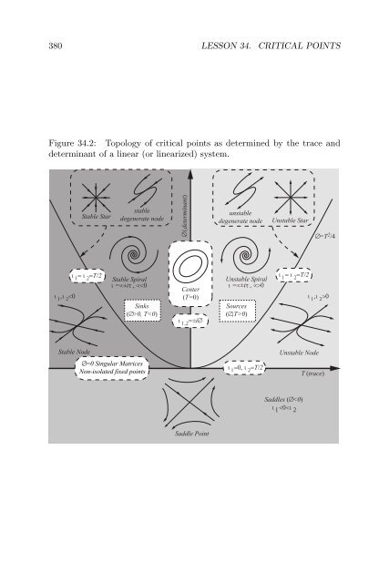
380 LESSON 34. CRITICAL POINTS Figure 34.2: Topology of critical points as determined by the trace and determinant of a linear (or linearized) system. Stable Star stable degenerate node determinant unstable degenerate node Unstable Star =T 2 /4 T/2 Stable Spiral =±i Sinks (>0, T0) T/2 Stable Node =0 Singular Matrices Non-isolated fixed points T/2 Unstable Node T (trace) Saddles (
381 Distinct Real Nonzero Eigenvalues of the Same Sign If T 2 > 4∆ > 0 both eigenvalues will be real and distinct. Repeated eigenvalues are excluded because T 2 ≠ 4∆. IfT > 0, both eigenvalues will both be positive, while if T < 0 both eigenvalues will be negative (note that T = 0 does not fall into this category). The solution is given by (34.48); A and B are determined by initial conditions. The special case A = B = 0 occurs only whenx(t 0 ) = y(t 0 ) = 0, which gives the isolated critical point at the origin. For nonzero initial conditions, the solution will be a linear combination of the two eigensolutions y 1 = ve λ1t (34.50) y 2 = we λ2t (34.51) By convention we will choose λ 1 to be the larger of the two eigenvalues in magnitude; then we will call the directions parallel to v and vthe fast eigendirection and the slow eigendirection, respectively. If both eigenvalues are positive, every solution becomes unbounded as t → ∞ (because e λit → ∞ as t → ∞) and approaches the origin as t → −∞ (because e λit → 0 as t → −∞), and the origin is called a source, repellor, or unstable node. If both eigenvalues are negative, the situation is reversed: every solution approaches the origin in positive time, as t → ∞, because e λit → 0 as t → ∞, and diverges in negative time as t → −∞ (because e λit → ∞ at t → −∞), and the origin is called a sink, attractor, or stable node. The names stable node and unstable node arise from the dynamical systems interpretation: a particle that is displaced an arbitrarily small distance away from the origin will move back towards the origin if it is a stable node, and will move further away from the origin if it is an unstable node. Despite the fact that the trajectories approach the origin either as t → ∞ or t → −∞, the only trajectory that actually passes through the origin is the isolated (single point) trajectory at the origin. Thus the only trajectory that passes through the origin is the one with A = B = 0. To see this consider the following. For a solution to intersect the origin at a time t would require Ave λ1t + Bwe λ2t = 0 (34.52)
- Page 337 and 338: 329 we find that ∫ M(t)g(t)dt = (
- Page 339 and 340: Lesson 32 The Laplace Transform Bas
- Page 341 and 342: 333 Figure 32.1: A piecewise contin
- Page 343 and 344: 335 Example 32.4. From integral A.1
- Page 345 and 346: 337 apply this result iteratively.
- Page 347 and 348: L [ t x−1] [ ] 1 d = L x dt tx =
- Page 349 and 350: 341 Equating numerators and expandi
- Page 351 and 352: 343 Derivatives of the Laplace Tran
- Page 353 and 354: 345 can be written as as illustrate
- Page 355 and 356: 347 Translations in the Laplace Var
- Page 357 and 358: 349 Summary of Translation Formulas
- Page 359 and 360: 351 The inverse transform is [ ] f(
- Page 361 and 362: 353 Example 32.18. Find the Laplace
- Page 363 and 364: 355 Similarly, we can express a uni
- Page 365 and 366: 357 Figure 32.7: Solution of exampl
- Page 367 and 368: Lesson 33 Numerical Methods Euler
- Page 369 and 370: 361 Figure 33.1: Illustration of Eu
- Page 371 and 372: 363 y 4 = y 3 + hf(t 3 , y 3 ) (33.
- Page 373 and 374: 365 Figure 33.3: Illustration of th
- Page 375 and 376: 367 result with a smaller step size
- Page 377 and 378: 369 Expanding the final term in a T
- Page 379 and 380: 371 k 2 = y 0 + h 2 f(t 0, k 1 ) (3
- Page 381 and 382: Lesson 34 Critical Points of Autono
- Page 383 and 384: 375 Since both f and g are differen
- Page 385 and 386: 377 Using the cos π/4 = √ 2/2 an
- Page 387: 379 values, of the matrix. We find
- Page 391 and 392: 383 eigendirection {λ 1 , v 1 }dom
- Page 393 and 394: 385 Figure 34.5: Phase portraits ty
- Page 395 and 396: 387 Complex Conjugate Pair with non
- Page 397 and 398: 389 The angular change is described
- Page 399 and 400: 391 Figure 34.8: Topological instab
- Page 401 and 402: 393 Figure 34.10: phase portraits f
- Page 403 and 404: Appendix A Table of Integrals Basic
- Page 405 and 406: 397 ∫ x √ x − adx = 2 3 a(x
- Page 407 and 408: 399 ∫ x √ ax2 + bx + c dx = 1 a
- Page 409 and 410: 401 ∫ ∫ ∫ ∫ e ax2 dx = −
- Page 411 and 412: 403 ∫ tan 3 axdx = 1 a ln cos ax
- Page 413 and 414: 405 Products of Trigonometric Funct
- Page 415 and 416: Appendix B Table of Laplace Transfo
- Page 417 and 418: 409 e at cosh kt t sin kt t cos kt
- Page 419 and 420: Appendix C Summary of Methods First
- Page 421 and 422: 413 The resulting equation is linea
- Page 423 and 424: 415 for y once z is known. Method o
- Page 425 and 426: Bibliography [1] Bear, H.S. Differe
- Page 427 and 428: BIBLIOGRAPHY 419
- Page 429 and 430: BIBLIOGRAPHY 421
380 LESSON 34. CRITICAL POINTS<br />
Figure 34.2: Topology of critical po<strong>in</strong>ts as determ<strong>in</strong>ed by the trace and<br />
determ<strong>in</strong>ant of a l<strong>in</strong>ear (or l<strong>in</strong>earized) system.<br />
Stable Star<br />
stable<br />
degenerate node<br />
determ<strong>in</strong>ant<br />
unstable<br />
degenerate node<br />
Unstable Star<br />
=T 2 /4<br />
<br />
T/2<br />
Stable Spiral<br />
=±i <br />
S<strong>in</strong>ks<br />
(>0, T0)<br />
T/2<br />
<br />
Stable Node<br />
=0 S<strong>in</strong>gular Matrices<br />
Non-isolated fixed po<strong>in</strong>ts<br />
T/2<br />
Unstable Node<br />
T (trace)<br />
Saddles (


