Lecture Notes in Differential Equations - Bruce E. Shapiro

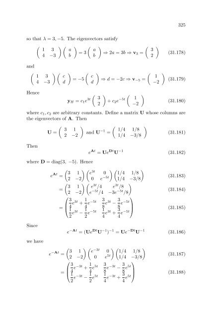
325
so that λ = 3, −5. The eigenvectors satisfy
( ) ( ) ( )
(
1 3 a a 3
= 3 ⇒ 2a = 3b ⇒ v
4 −3 b b
3 =
2
)
(31.178)
and
(
1 3
4 −3
) (
c
d
)
( c
= −5
d
)
( 1
⇒ d = −2c ⇒ v −5 =
−2
)
(31.179)
Hence
y H = c 1 e 3t (
3
2
)
+ c 2 e −5t (
1
−2
)
(31.180)
where c 1 , c 2 are arbitrary constants. Define a matrix U whose columns are
the eigenvectors of A. Then
Then
U =
( 3 1
2 −2
)
where D = diag(3, −5). Hence
and U −1 =
( 1/4 1/8
1/4 −3/8
)
(31.181)
e At = Ue Dt U −1 (31.182)
( ) ( ) ( )
e At 3 1 e
3t
0 1/4 1/8
=
2 −2 0 e −5t (31.183)
1/4 −3/8
( ) ( )
3 1 e
=
3t /4 e 3t /8
2 −2 e −5t /4 −3e −5t (31.184)
/8
⎛
3
⎜
= ⎝4 e3t + 1 3
4 e−5t 8 e3t − 3 ⎞
8 e−5t
1
2 e3t − 1 1
2 e−5t 4 e3t + 3 ⎟
⎠ (31.185)
4 e−5t
Since
we have
e −At = (Ue Dt U −1 ) −1 = Ue −Dt U −1 (31.186)
( ) ( ) ( )
e −At 3 1 e
−3t
0 1/4 1/8
=
2 −2 0 e 5t (31.187)
1/4 −3/8
⎛
3
⎜
= ⎝4 e−3t + 1 3
4 e5t 8 e−3t − 3 ⎞
8 e5t
1
2 e−3t − 1 1
2 e5t 4 e−3t + 3 ⎟
⎠ (31.188)
4 e5t