- Page 1 and 2:
Lecture Notes in Differential Equat
- Page 3 and 4:
Contents Front Cover . . . . . . .
- Page 5 and 6:
CONTENTS v Dedicated to the hundred
- Page 7 and 8:
Preface These lecture notes on diff
- Page 9 and 10:
Lesson 1 Basic Concepts A different
- Page 11 and 12:
3 Definition 1.2 (Solution, ODE). A
- Page 13 and 14:
5 1.22 is restricted to being a pos
- Page 15 and 16:
7 Figure 1.1 illustrates what this
- Page 17 and 18:
9 We will study linear equations in
- Page 19 and 20:
Lesson 2 A Geometric View One way t
- Page 21 and 22:
13 We can extend this geometric int
- Page 23 and 24:
15 that since the slope of the solu
- Page 25 and 26:
Lesson 3 Separable Equations An ODE
- Page 27 and 28:
19 Since it is not possible to solv
- Page 29 and 30:
21 where M(t) = −a(t) and N(y) =
- Page 31 and 32:
23 Example 3.10. Find a general sol
- Page 33 and 34:
Lesson 4 Linear Equations Recall th
- Page 35 and 36:
27 So far any function µ will work
- Page 37 and 38:
29 Example 4.1. Solve the different
- Page 39 and 40:
31 Since p(t) = 1 (the coefficient
- Page 41 and 42:
33 Multiplying equation 4.68 by µ
- Page 43 and 44:
35 Substituting y = t = 0 in this i
- Page 45 and 46:
37 ∫ t t 0 Evaluating the integra
- Page 47 and 48:
Lesson 5 Bernoulli Equations The Be
- Page 49 and 50:
41 This is a Bernoulli equation wit
- Page 51 and 52:
Lesson 6 Exponential Relaxation One
- Page 53 and 54:
45 Exponential Runaway First we con
- Page 55 and 56:
47 Figure 6.2: Illustration of the
- Page 57 and 58:
49 This is identical to with Theref
- Page 59 and 60:
51 this becomes a first-order ODE i
- Page 61 and 62:
Lesson 7 Autonomous Differential Eq
- Page 63 and 64:
55 Figure 7.1: A plot of the right-
- Page 65 and 66:
57 Figure 7.2: Solutions of the log
- Page 67 and 68:
59 Figure 7.4: Solutions of the thr
- Page 69 and 70:
Lesson 8 Homogeneous Equations Defi
- Page 71 and 72:
63 where z = y/t, the differential
- Page 73 and 74:
Lesson 9 Exact Equations We can re-
- Page 75 and 76:
67 Now compare equation (9.2) with
- Page 77 and 78:
69 Hence dg dy = 0 =⇒ g = C′ (9
- Page 79 and 80:
71 From the first of equations (9.5
- Page 81 and 82:
73 Differentiating equations (9.81)
- Page 83 and 84:
75 This has the form Mdt + Ndy = 0
- Page 85 and 86:
Lesson 10 Integrating Factors Defin
- Page 87 and 88:
79 Differentiating with respect to
- Page 89 and 90:
81 Proof. In each of the five cases
- Page 91 and 92:
83 as required by equation (10.31).
- Page 93 and 94:
85 Since M y ≠ N t , equation (10
- Page 95 and 96:
87 the revised equation (10.100) is
- Page 97 and 98:
89 Substituting (10.129) into (10.1
- Page 99 and 100:
Lesson 11 Method of Successive Appr
- Page 101 and 102:
93 because the integral is zero (th
- Page 103 and 104:
95 Example 11.1. Construct the Pica
- Page 105 and 106:
97 We can then plug this expression
- Page 107 and 108:
Lesson 12 Existence of Solutions* I
- Page 109 and 110:
101 • Interchangeability of Limit
- Page 111 and 112:
103 But on the square −1 ≤ t
- Page 113 and 114:
105 Thus lim φ n = φ 0 + lim n→
- Page 115 and 116:
107 because the right hand side doe
- Page 117 and 118:
Lesson 13 Uniqueness of Solutions*
- Page 119 and 120:
111 The proof of theorem (13.1) is
- Page 121 and 122:
113 But δ(t) is an absolute value,
- Page 123 and 124:
115 Substituting (13.66) into (13.6
- Page 125 and 126:
Lesson 14 Review of Linear Algebra
- Page 127 and 128:
119 Definition 14.10. An m × n (or
- Page 129 and 130:
121 Definition 14.19. Matrix Multip
- Page 131 and 132:
123 In practical terms, computation
- Page 133 and 134:
125 Simplifying 4x − 2 + 3z = 0 (
- Page 135 and 136:
Lesson 15 Linear Operators and Vect
- Page 137 and 138:
129 Example 15.3. By a similar argu
- Page 139 and 140:
131 Therefore ‖y + z‖ 2 ≤ ‖
- Page 141 and 142:
133 Definition 15.5. Two vectors y,
- Page 143 and 144:
Lesson 16 Linear Equations With Con
- Page 145 and 146:
137 Hence both r = 1 and r = 3. Thi
- Page 147 and 148:
139 The second order linear initial
- Page 149 and 150:
141 The general solution to is give
- Page 151 and 152:
Lesson 17 Some Special Substitution
- Page 153 and 154:
145 Therefore since z = y ′ , Int
- Page 155 and 156:
147 Example 17.5. Solve yy ′′ +
- Page 157 and 158:
149 where I is the identity matrix.
- Page 159 and 160:
151 can be rewritten by solving a =
- Page 161 and 162:
Lesson 18 Complex Roots We know for
- Page 163 and 164:
155 Theorem 18.2. Euler’s Formula
- Page 165 and 166:
157 For k = 0, 1, 2, . . . , n −
- Page 167 and 168:
159 and its roots are given by The
- Page 169 and 170:
161 The motivation for equation 18.
- Page 171 and 172:
Lesson 19 Method of Undetermined Co
- Page 173 and 174:
165 3. If f(t) = e rt and r is a ro
- Page 175 and 176:
167 Example 19.4. Solve ⎫ y ′
- Page 177 and 178:
169 Adding the two equations gives
- Page 179 and 180:
Lesson 20 The Wronskian We have see
- Page 181 and 182:
173 Definition 20.1. The Wronskian
- Page 183 and 184:
175 Example 20.3. Show that y = sin
- Page 185 and 186:
177 and therefore the system of equ
- Page 187 and 188:
Lesson 21 Reduction of Order The me
- Page 189 and 190:
181 The method of reduction of orde
- Page 191 and 192:
183 Plugging these into Bessel’s
- Page 193 and 194:
185 Example 21.5. Find a second sol
- Page 195 and 196:
Lesson 22 Non-homogeneous Equations
- Page 197 and 198:
189 where r 1 and r 2 are the roots
- Page 199 and 200:
191 This is a first order linear eq
- Page 201 and 202:
193 Theorem 22.5. Properties of the
- Page 203 and 204:
195 where (∫ ν(t) = exp ) −r 2
- Page 205 and 206:
197 The characteristic equation is
- Page 207 and 208:
Lesson 23 Method of Annihilators In
- Page 209 and 210:
201 Theorem 23.5. (D 2 − 2aD + (a
- Page 211 and 212: 203 The method of annihilators is r
- Page 213 and 214: Lesson 24 Variation of Parameters T
- Page 215 and 216: 207 Substituting into equation (24.
- Page 217 and 218: 209 Example 24.3. Solve the initial
- Page 219 and 220: Lesson 25 Harmonic Oscillations If
- Page 221 and 222: 213 It is standard to define a new
- Page 223 and 224: 215 As with the unforced case, we c
- Page 225 and 226: Lesson 26 General Existence Theory*
- Page 227 and 228: 219 In the case just proven, there
- Page 229 and 230: 221 Theorem 26.5. Under the same co
- Page 231 and 232: 223 Since K n /(1 − K) → 0 as n
- Page 233 and 234: 225 for any φ ∈ V. Let g, h be f
- Page 235 and 236: Lesson 27 Higher Order Linear Equat
- Page 237 and 238: 229 L n+1 (e rt y) = e rt a n (D +
- Page 239 and 240: 231 Example 27.2. Find the general
- Page 241 and 242: 233 Differentiating, u ′ (t) = d
- Page 243 and 244: 235 Integrating, − 2K |t − t 0
- Page 245 and 246: 237 a closed form expression for a
- Page 247 and 248: 239 Example 27.6. Find the general
- Page 249 and 250: 241 The characteristic equation is
- Page 251 and 252: 243 The Wronskian In this section w
- Page 253 and 254: 245 Certainly every φ(t) given by
- Page 255 and 256: 247 the differential equation. Over
- Page 257 and 258: 249 By the lemma, to obtain the der
- Page 259 and 260: 251 Example 27.14. Find the general
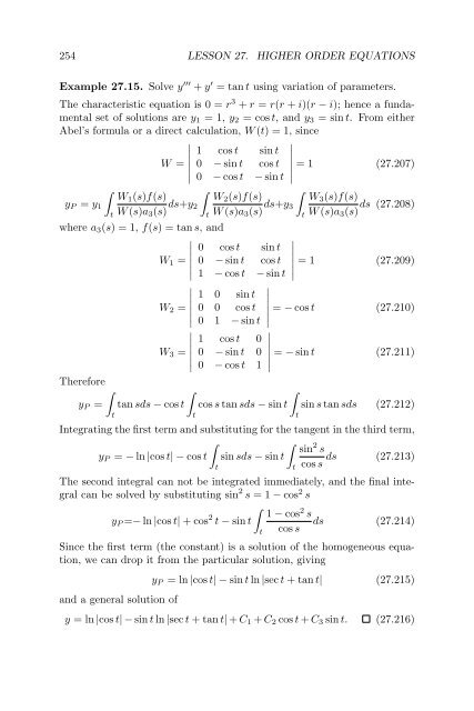
- Page 261: 253 So that f(t) = a n (t)y[ (n) +
- Page 265 and 266: 257 Changing the index of the secon
- Page 267 and 268: 259 Since the first two terms (corr
- Page 269 and 270: 261 Hence ∞∑ ∞∑ ∞∑ 0 =
- Page 271 and 272: 263 has an analytic solution at t =
- Page 273 and 274: 265 By the triangle inequality, |(k
- Page 275 and 276: 267 Table 28.1: Table of Special Fu
- Page 277 and 278: 269 Thus y = a 0 ( 1 + 1 6 t3 + 1 +
- Page 279 and 280: 271 into (28.114) and collect terms
- Page 281 and 282: 273 Summary of Power series method.
- Page 283 and 284: Lesson 29 Regular Singularities The
- Page 285 and 286: 277 ∑ ∞ ∞∑ ∞∑ 0 = t 2 a
- Page 287 and 288: 279 Case 2: Two equal real roots. S
- Page 289 and 290: 281 Example 29.6. Solve t 2 y ′
- Page 291 and 292: Lesson 30 The Method of Frobenius I
- Page 293 and 294: 285 This is a homogeneous linear eq
- Page 295 and 296: 287 Example 30.4. Find a Frobenius
- Page 297 and 298: 289 Thus a Frobenius solution is y
- Page 299 and 300: 291 Example 30.6. Find the form of
- Page 301 and 302: 293 term by term to (30.97). Starti
- Page 303 and 304: 295 Let j = n − k. Then |n − 1
- Page 305 and 306: 297 is a solution of (t − t 0 ) 2
- Page 307 and 308: 299 Evaluation of the integral depe
- Page 309 and 310: 301 Example 30.8. In example 30.4 w
- Page 311 and 312: Lesson 31 Linear Systems The genera
- Page 313 and 314:
305 is where λ 2 − T λ + ∆ =
- Page 315 and 316:
307 (b) If λ 1 ≠ λ 2 ∈ R, i.e
- Page 317 and 318:
309 We will verify (31.54) by induc
- Page 319 and 320:
311 The Jordan Form Let A be a squa
- Page 321 and 322:
313 y = 1 [( ) ( ) ] ( ) 4 1 e 2t 1
- Page 323 and 324:
315 Theorem 31.8. (Abel’s Formula
- Page 325 and 326:
317 By a similar argument, the seco
- Page 327 and 328:
319 we can replace (31.118) with a
- Page 329 and 330:
321 Corollary 31.12. The generalize
- Page 331 and 332:
323 where (A − λI)w 2 = w 1 , i.
- Page 333 and 334:
325 so that λ = 3, −5. The eigen
- Page 335 and 336:
327 Non-constant Coefficients We ca
- Page 337 and 338:
329 we find that ∫ M(t)g(t)dt = (
- Page 339 and 340:
Lesson 32 The Laplace Transform Bas
- Page 341 and 342:
333 Figure 32.1: A piecewise contin
- Page 343 and 344:
335 Example 32.4. From integral A.1
- Page 345 and 346:
337 apply this result iteratively.
- Page 347 and 348:
L [ t x−1] [ ] 1 d = L x dt tx =
- Page 349 and 350:
341 Equating numerators and expandi
- Page 351 and 352:
343 Derivatives of the Laplace Tran
- Page 353 and 354:
345 can be written as as illustrate
- Page 355 and 356:
347 Translations in the Laplace Var
- Page 357 and 358:
349 Summary of Translation Formulas
- Page 359 and 360:
351 The inverse transform is [ ] f(
- Page 361 and 362:
353 Example 32.18. Find the Laplace
- Page 363 and 364:
355 Similarly, we can express a uni
- Page 365 and 366:
357 Figure 32.7: Solution of exampl
- Page 367 and 368:
Lesson 33 Numerical Methods Euler
- Page 369 and 370:
361 Figure 33.1: Illustration of Eu
- Page 371 and 372:
363 y 4 = y 3 + hf(t 3 , y 3 ) (33.
- Page 373 and 374:
365 Figure 33.3: Illustration of th
- Page 375 and 376:
367 result with a smaller step size
- Page 377 and 378:
369 Expanding the final term in a T
- Page 379 and 380:
371 k 2 = y 0 + h 2 f(t 0, k 1 ) (3
- Page 381 and 382:
Lesson 34 Critical Points of Autono
- Page 383 and 384:
375 Since both f and g are differen
- Page 385 and 386:
377 Using the cos π/4 = √ 2/2 an
- Page 387 and 388:
379 values, of the matrix. We find
- Page 389 and 390:
381 Distinct Real Nonzero Eigenvalu
- Page 391 and 392:
383 eigendirection {λ 1 , v 1 }dom
- Page 393 and 394:
385 Figure 34.5: Phase portraits ty
- Page 395 and 396:
387 Complex Conjugate Pair with non
- Page 397 and 398:
389 The angular change is described
- Page 399 and 400:
391 Figure 34.8: Topological instab
- Page 401 and 402:
393 Figure 34.10: phase portraits f
- Page 403 and 404:
Appendix A Table of Integrals Basic
- Page 405 and 406:
397 ∫ x √ x − adx = 2 3 a(x
- Page 407 and 408:
399 ∫ x √ ax2 + bx + c dx = 1 a
- Page 409 and 410:
401 ∫ ∫ ∫ ∫ e ax2 dx = −
- Page 411 and 412:
403 ∫ tan 3 axdx = 1 a ln cos ax
- Page 413 and 414:
405 Products of Trigonometric Funct
- Page 415 and 416:
Appendix B Table of Laplace Transfo
- Page 417 and 418:
409 e at cosh kt t sin kt t cos kt
- Page 419 and 420:
Appendix C Summary of Methods First
- Page 421 and 422:
413 The resulting equation is linea
- Page 423 and 424:
415 for y once z is known. Method o
- Page 425 and 426:
Bibliography [1] Bear, H.S. Differe
- Page 427 and 428:
BIBLIOGRAPHY 419
- Page 429 and 430:
BIBLIOGRAPHY 421