Lecture Notes in Differential Equations - Bruce E. Shapiro

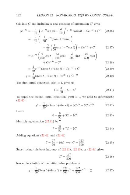
192 LESSON 22. NON-HOMOG. EQS.W/ CONST. COEFF.
this into C and including a new constant of integration C ′ gives
ye −7t = − 9 ∫
e −7t sin tdt − 3 ∫
e −7t cos ttdt + Ce −4t + C ′ (22.36)
10
10
= − 9 (
− 1 )
10 50 e−7t (cos t + 7 sin t)
− 3 ( )
1
10 50 (sin t − 7 cos t) + Ce −4t + C ′ (22.37)
( 9
= e −7t 63
cos t +
500 500 sin t − 3
)
21
sin t +
500 500 cos t
+ Ce −4t + C ′ (22.38)
= 1
50 e−7t (3 cos t + 6 sin t) + Ce −4t + C ′ (22.39)
y = 1
50 (3 cos t + 6 sin t) + Ce3t + C ′ e −7t (22.40)
The first initial condition, y(0) = 1, gives us
1 = 3
50 + C + C′ (22.41)
To apply the second initial condition, y ′ (0) = 0, we need to differentiate
(22.40)
y ′ = 1
50 (−3 sin t + 6 cos t) + 3Ce3t − 7C ′ e −7t (22.42)
Hence
0 = 6 50 + 3C − 7C′ (22.43)
Multiplying equation (22.41) by 7
Adding equations (22.43) and (22.44)
7 = 21
50 + 7C + 7C′ (22.44)
7 = 27
323
+ 10C =⇒ C =
50 500
Substituting this back into any of (22.41), (22.43), or (22.44) gives
C ′ = 147
500
hence the solution of the initial value problem is
(22.45)
(22.46)
y = 1
323
(3 cos t + 6 sin t) +
50 500 e3t + 147
500 e−7t (22.47)