Lecture Notes in Differential Equations - Bruce E. Shapiro
Lecture Notes in Differential Equations - Bruce E. Shapiro Lecture Notes in Differential Equations - Bruce E. Shapiro
182 LESSON 21. REDUCTION OF ORDER Substitution back into the original ODE verifies that this works. Hence a general solution of the equation is ∫ y = At + Bt t −2 e −t2 /2 dt (21.35) Example 21.3. Find a second solution of t 2 y ′′ − 4ty ′ + 6y = 0 (21.36) assuming that t > 0, given that y 1 = t 2 is already a solution. We look for a solution of the form y 2 = uy 1 = ut 2 . Differentiating Substituting in (21.36), y ′ 2 = u ′ t 2 + 2tu (21.37) y ′′ 2 = u ′′ t 2 + 4tu ′ + 2u (21.38) 0 = t 2 (u ′′ t 2 + 4tu ′ + 2u) − 4t(u ′ t 2 + 2tu) + 6ut 2 (21.39) = t 4 u ′′ + 4t 3 u ′ + 2t 2 u − 4t 3 u ′ − 8t 2 u + 6t 2 u (21.40) = t 4 u ′′ (21.41) Since t > 0 we can never have t = 0; hence we can divide by t 4 to give u ′′ = 0. This means u = t. Hence y 2 = uy 1 = t 3 (21.42) is a second solution. Example 21.4. Show that y 1 = sin t √ t (21.43) is a solution of Bessel’s equation of order 1/2 ( t 2 y ′′ + ty ′ + t 2 − 1 ) y = 0 (21.44) 4 and use reduction of order to find a second solution. Differentiating using the product rule y 1 ′ = d ( ) t −1/2 sin t dt (21.45) = t −1/2 cos t − 1 2 t−3/2 sin t (21.46) y ′′ 1 = −t −1/2 sin t − t −3/2 cos t + 3 4 t−5/2 sin t (21.47)
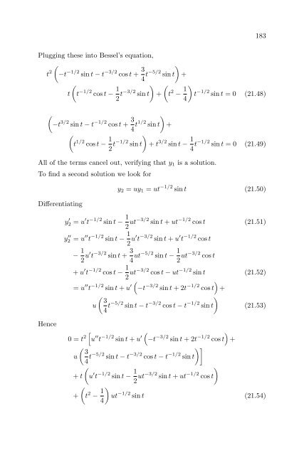
183 Plugging these into Bessel’s equation, t (−t 2 −1/2 sin t − t −3/2 cos t + 3 ) 4 t−5/2 sin t + ( t t −1/2 cos t − 1 ) ( 2 t−3/2 sin t + t 2 − 1 ) t −1/2 sin t = 0 (21.48) 4 ( −t 3/2 sin t − t −1/2 cos t + 3 ) 4 t1/2 sin t + ( t 1/2 cos t − 1 ) 2 t−1/2 sin t + t 3/2 sin t − 1 4 t−1/2 sin t = 0 (21.49) All of the terms cancel out, verifying that y 1 is a solution. To find a second solution we look for Differentiating y 2 = uy 1 = ut −1/2 sin t (21.50) y ′ 2 = u ′ t −1/2 sin t − 1 2 ut−3/2 sin t + ut −1/2 cos t (21.51) y ′′ 2 = u ′′ t −1/2 sin t − 1 2 u′ t −3/2 sin t + u ′ t −1/2 cos t − 1 2 u′ t −3/2 sin t + 3 4 ut−5/2 sin t − 1 2 ut−3/2 cos t + u ′ t −1/2 cos t − 1 2 ut−3/2 cos t − ut −1/2 sin t (21.52) ( ) = u ′′ t −1/2 sin t + u ′ −t −3/2 sin t + 2t −1/2 cos t + ( ) 3 u 4 t−5/2 sin t − t −3/2 cos t − t −1/2 sin t (21.53) Hence [ ( ) 0 = t 2 u ′′ t −1/2 sin t + u ′ −t −3/2 sin t + 2t −1/2 cos t + ( )] 3 u 4 t−5/2 sin t − t −3/2 cos t − t −1/2 sin t ( + t u ′ t −1/2 sin t − 1 ) 2 ut−3/2 sin t + ut −1/2 cos t ( + t 2 − 1 ) ut −1/2 sin t (21.54) 4
- Page 139 and 140: 131 Therefore ‖y + z‖ 2 ≤ ‖
- Page 141 and 142: 133 Definition 15.5. Two vectors y,
- Page 143 and 144: Lesson 16 Linear Equations With Con
- Page 145 and 146: 137 Hence both r = 1 and r = 3. Thi
- Page 147 and 148: 139 The second order linear initial
- Page 149 and 150: 141 The general solution to is give
- Page 151 and 152: Lesson 17 Some Special Substitution
- Page 153 and 154: 145 Therefore since z = y ′ , Int
- Page 155 and 156: 147 Example 17.5. Solve yy ′′ +
- Page 157 and 158: 149 where I is the identity matrix.
- Page 159 and 160: 151 can be rewritten by solving a =
- Page 161 and 162: Lesson 18 Complex Roots We know for
- Page 163 and 164: 155 Theorem 18.2. Euler’s Formula
- Page 165 and 166: 157 For k = 0, 1, 2, . . . , n −
- Page 167 and 168: 159 and its roots are given by The
- Page 169 and 170: 161 The motivation for equation 18.
- Page 171 and 172: Lesson 19 Method of Undetermined Co
- Page 173 and 174: 165 3. If f(t) = e rt and r is a ro
- Page 175 and 176: 167 Example 19.4. Solve ⎫ y ′
- Page 177 and 178: 169 Adding the two equations gives
- Page 179 and 180: Lesson 20 The Wronskian We have see
- Page 181 and 182: 173 Definition 20.1. The Wronskian
- Page 183 and 184: 175 Example 20.3. Show that y = sin
- Page 185 and 186: 177 and therefore the system of equ
- Page 187 and 188: Lesson 21 Reduction of Order The me
- Page 189: 181 The method of reduction of orde
- Page 193 and 194: 185 Example 21.5. Find a second sol
- Page 195 and 196: Lesson 22 Non-homogeneous Equations
- Page 197 and 198: 189 where r 1 and r 2 are the roots
- Page 199 and 200: 191 This is a first order linear eq
- Page 201 and 202: 193 Theorem 22.5. Properties of the
- Page 203 and 204: 195 where (∫ ν(t) = exp ) −r 2
- Page 205 and 206: 197 The characteristic equation is
- Page 207 and 208: Lesson 23 Method of Annihilators In
- Page 209 and 210: 201 Theorem 23.5. (D 2 − 2aD + (a
- Page 211 and 212: 203 The method of annihilators is r
- Page 213 and 214: Lesson 24 Variation of Parameters T
- Page 215 and 216: 207 Substituting into equation (24.
- Page 217 and 218: 209 Example 24.3. Solve the initial
- Page 219 and 220: Lesson 25 Harmonic Oscillations If
- Page 221 and 222: 213 It is standard to define a new
- Page 223 and 224: 215 As with the unforced case, we c
- Page 225 and 226: Lesson 26 General Existence Theory*
- Page 227 and 228: 219 In the case just proven, there
- Page 229 and 230: 221 Theorem 26.5. Under the same co
- Page 231 and 232: 223 Since K n /(1 − K) → 0 as n
- Page 233 and 234: 225 for any φ ∈ V. Let g, h be f
- Page 235 and 236: Lesson 27 Higher Order Linear Equat
- Page 237 and 238: 229 L n+1 (e rt y) = e rt a n (D +
- Page 239 and 240: 231 Example 27.2. Find the general
183<br />
Plugg<strong>in</strong>g these <strong>in</strong>to Bessel’s equation,<br />
t<br />
(−t 2 −1/2 s<strong>in</strong> t − t −3/2 cos t + 3 )<br />
4 t−5/2 s<strong>in</strong> t +<br />
(<br />
t t −1/2 cos t − 1 ) (<br />
2 t−3/2 s<strong>in</strong> t + t 2 − 1 )<br />
t −1/2 s<strong>in</strong> t = 0 (21.48)<br />
4<br />
(<br />
−t 3/2 s<strong>in</strong> t − t −1/2 cos t + 3 )<br />
4 t1/2 s<strong>in</strong> t +<br />
(<br />
t 1/2 cos t − 1 )<br />
2 t−1/2 s<strong>in</strong> t + t 3/2 s<strong>in</strong> t − 1 4 t−1/2 s<strong>in</strong> t = 0 (21.49)<br />
All of the terms cancel out, verify<strong>in</strong>g that y 1 is a solution.<br />
To f<strong>in</strong>d a second solution we look for<br />
Differentiat<strong>in</strong>g<br />
y 2 = uy 1 = ut −1/2 s<strong>in</strong> t (21.50)<br />
y ′ 2 = u ′ t −1/2 s<strong>in</strong> t − 1 2 ut−3/2 s<strong>in</strong> t + ut −1/2 cos t (21.51)<br />
y ′′<br />
2 = u ′′ t −1/2 s<strong>in</strong> t − 1 2 u′ t −3/2 s<strong>in</strong> t + u ′ t −1/2 cos t<br />
− 1 2 u′ t −3/2 s<strong>in</strong> t + 3 4 ut−5/2 s<strong>in</strong> t − 1 2 ut−3/2 cos t<br />
+ u ′ t −1/2 cos t − 1 2 ut−3/2 cos t − ut −1/2 s<strong>in</strong> t (21.52)<br />
( )<br />
= u ′′ t −1/2 s<strong>in</strong> t + u ′ −t −3/2 s<strong>in</strong> t + 2t −1/2 cos t +<br />
( )<br />
3<br />
u<br />
4 t−5/2 s<strong>in</strong> t − t −3/2 cos t − t −1/2 s<strong>in</strong> t (21.53)<br />
Hence<br />
[ ( )<br />
0 = t 2 u ′′ t −1/2 s<strong>in</strong> t + u ′ −t −3/2 s<strong>in</strong> t + 2t −1/2 cos t +<br />
( )]<br />
3<br />
u<br />
4 t−5/2 s<strong>in</strong> t − t −3/2 cos t − t −1/2 s<strong>in</strong> t<br />
(<br />
+ t u ′ t −1/2 s<strong>in</strong> t − 1 )<br />
2 ut−3/2 s<strong>in</strong> t + ut −1/2 cos t<br />
(<br />
+ t 2 − 1 )<br />
ut −1/2 s<strong>in</strong> t (21.54)<br />
4


