Lecture Notes in Differential Equations - Bruce E. Shapiro

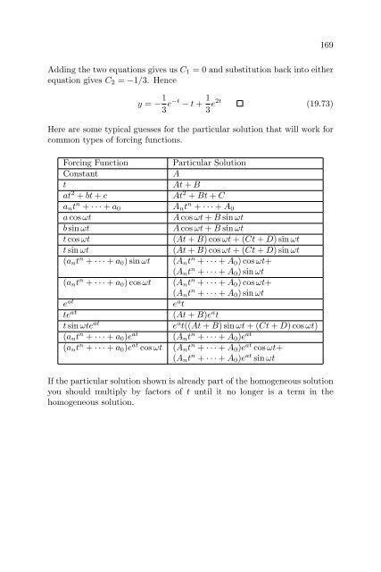
169
Adding the two equations gives us C 1 = 0 and substitution back into either
equation gives C 2 = −1/3. Hence
y = − 1 3 e−t − t + 1 3 e2t (19.73)
Here are some typical guesses for the particular solution that will work for
common types of forcing functions.
Forcing Function
Particular Solution
Constant
A
t
At + B
at 2 + bt + c
At 2 + Bt + C
a n t n + · · · + a 0 A n t n + · · · + A 0
a cos ωt
A cos ωt + B sin ωt
b sin ωt
A cos ωt + B sin ωt
t cos ωt
(At + B) cos ωt + (Ct + D) sin ωt
t sin ωt
(At + B) cos ωt + (Ct + D) sin ωt
(a n t n + · · · + a 0 ) sin ωt (A n t n + · · · + A 0 ) cos ωt+
(A n t n + · · · + A 0 ) sin ωt
(a n t n + · · · + a 0 ) cos ωt (A n t n + · · · + A 0 ) cos ωt+
(A n t n + · · · + A 0 ) sin ωt
e at
e a t
te at
(At + B)e a t
t sin ωte at
e a t((At + B) sin ωt + (Ct + D) cos ωt)
(a n t n + · · · + a 0 )e at (A n t n + · · · + A 0 )e at
(a n t n + · · · + a 0 )e at cos ωt (A n t n + · · · + A 0 )e at cos ωt+
(A n t n + · · · + A 0 )e at sin ωt
If the particular solution shown is already part of the homogeneous solution
you should multiply by factors of t until it no longer is a term in the
homogeneous solution.