2 Sediment and Pollutant Transport - Basement - ETH ZÃ¼rich

System Manuals of BASEMENT 

CREDITS 

VERSION 1.1 

October, 2006 

Project Team 

Prof. Dr.-Ing. H.-E. Minor, 

Member of the steering committee of Rhone-Thur Project, Director VAW 

Dr. R. Fäh, Dipl. Ing. ETH 

Module manager within Rhone-Thur Project, Scientific supervisor BASEMENT 

Dr.-Ing. D. Farshi, M. Sc., Software development BASEplane, Scientific Associate 

R. Müller, Dipl. Ing. EPFL, Software development BASEchain, Scientific Associate 

P. Rousselot, Dipl. Rech. Wiss. ETH, Software development, Scientific Associate 

D. Vetsch, Dipl. Ing. ETH, Project Supervisor BASEMENT, Scientific Associate 

Art Design and Layout 

W. Thürig, D. Vetsch 

Lectorate 

Dr. U. Keller 

Commissioned and co-financed by 

Swiss Federal Office 

for the Environment (FOEN) 

Contact 

basement@ethz.ch 

http://www.basement.ethz.ch 

© ETH Zurich, VAW, Faeh R., Farshi D., Mueller R., Rousselot P., Vetsch D., 2006 

VAW ETH Zürich 

Version 10/4/2006


PREFACE 

Preface 

The development of computer programs for solving demanding hydraulic or hydrological 

problems has an almost thirty-year tradition at VAW. Many projects have been carried out 

with the application of “home-made” numerical codes and were successfully finished. The 

according software development and its applications were primarily promoted by the 

individual initiative of scientific associates of VAW and financed by federal instances or the 

private sector. Most often, the programs were tailored for a specific application and adapted 

to fulfil costumer needs. Consequently, the software grew in functionality but with little 

documentation. Due to limited temporal and personal resources to absolve an according 

project, a single point of knowledge concerning the details of the software was inevitable in 

most of the cases. 

In 2002, the applied numerics group of VAW was invited by the Swiss federal office for 

water and geology (BWG, nowadays Swiss Federal Office for the Environment FOEN) to 

offer for participation in the trans-disciplinary “Rhone-Thur” project. With the idea to build up 

a new software tool based on the knowledge gained by former numerical codes - while 

eliminating their shortcomings and expanding their functionality - a proposal was submitted. 

The bidding being successful a partnership in terms of co-financing was established. By the 

end of 2002, a newly formed team took up the work to build the so-called “BASic 

EnvironMENT for simulation of environmental flow and natural hazard simulation – 

BASEMENT”. 

From the beginning, the objectives for the new project were ambitious: developing a 

software system from scratch, containing all the experience of many years as well as stateof-the-art 

numerics with general applicability and providing the ability to simulate sediment 

transport. Additionally, professional documentation is a must. As to meet all these demands, 

a part wise reengineering of existing codes (Floris, 2dmb) has been carried out, while 

merging it with modern and new numerical approaches. From a software-technical point of 

view, an object-oriented approach has been chosen, with the aim to provide reusability, 

reliability, robustness, extensibility and maintainability of the software to be developed. 

After four years of designing, implementing and testing, the software system BASEMENT 

has reached a state to go public. The documentation at hand confirms the invested diligence 

to create a transparent software system of high quality. The software, in terms of an 

executable computer program, and its documentation are available free of charge. It can be 

used by anyone who wants to run numerical simulations of rivers and sediment transport – 

either for training or for commercial purposes. 


Version 10/5/2006


PREFACE 

The further development of the software tends to new approaches for sediment transport 

simulation, carried out within the scope of scientific studies on one hand side. On the other 

hand, effectiveness and composite modelling are the goals. On either side, a reliable 

software system BASEMENT will have to meet expectations of the practical engineer and 

the scientist at the same time. 

Prof. Dr.-Ing. H.-E. Minor 

Member of the steering committee of Rhone-Thur Project, Director VAW 

October, 2006 


Version 10/5/2006


LICENSE AGREEMENT 

1. Definition of the Software 

SOFTWARE LICENSE 

between 

ETH Zurich 

Rämistrasse 101 

8092 Zürich 

Represented by Prof. Hans Erwin Minor 

VAW 

(Licensor) 

and 

Licensee 

The Software system BASEMENT is composed of the executable (binary) files BASEMENT, BASEchain and 

BASEplane and its documentation files (System Manuals), together herein after referred to as “Software”. Not 

included is the source code. 

Its purpose is the simulation of water flow, sediment and pollutant transport and according interaction in 

consideration of movable boundaries and morphological changes. 

2. License of ETH Zurich 

ETH Zurich hereby grants a single, non-exclusive, world-wide, royalty-free license to use Software to the licensee 

subject to all the terms and conditions of this Agreement. 

3. The scope of the license 

a. Use 

The licensee may use the Software: 

- according to the intended purpose of the Software as defined in provision 1 

- by the licensee and his employees 

- for commercial and non-commercial purposes 

The generation of essential temporary backups is allowed. 

b. Reproduction / Modification 

Neither reproduction (other than plain backup copies) nor modification is permitted with the following 

exceptions: 

Decoding according to article 21 URG [Bundesgesetz über das Urheberrecht, SR 231.1) 

If the licensee intends to access the program with other interoperative programs according to article 21 URG, he 

is to contact licensor explaining his requirement. 

If the licensor neither provides according support for the interoperative programs nor makes the necessary 

source code available within 30 days, licensee is entitled, after reminding the licensor once, to obtain the 

information for the above mentioned intentions by source code generation through decompilation. 

c. Adaptation 

On his own risk, the licensee has the right to parameterize the Software or to access the Software with 

interoperable programs within the aforementioned scope of the licence. 

d. Distribution of Software to sub licensees 

Licensee may transfer this Software in its original form to sub licensees. Sub licensees have to agree to all 

terms and conditions of this Agreement. It is prohibited to impose any further restrictions on the sub licensees’ 

exercise of the rights granted herein. 

No fees may be charged for use, reproduction, modification or distribution of this Software, neither in 

unmodified nor incorporated forms, with the exception of a fee for the physical act of transferring a copy or for 

an additional warranty protection. 

4. Obligations of licensee 

a. Copyright Notice 

Software as well as interactively generated output must conspicuously and appropriately quote the following 

copyright notices: 

Copyright by ETH Zurich, VAW, Faeh Roland, Farshi Davood, Mueller Renata, Rousselot Patric, Vetsch David, 2006 


Version 10/6/2006


LICENSE AGREEMENT 

5. Intellectual property and other rights 

The licensee obtains all rights granted in this Agreement and retains all rights to results from the use of the 

Software. 

Ownership, intellectual property rights and all other rights in and to the Software shall remain with ETH Zurich 

(licensor). 

6. Installation, maintenance, support, upgrades or new releases 

a. Installation 

The licensee may download the Software from the web page http://www.basement.ethz.ch or access it from 

the distributed CD. 

b. Maintenance, support, upgrades or new releases 

ETH Zurich doesn’t have any obligation of maintenance, support, upgrades or new releases, and disclaims all 

costs associated with service, repair or correction. 

7. Warranty 

ETH Zurich does not make any warranty concerning the: 

- warranty of merchantability, satisfactory quality and fitness for a particular purpose 

- warranty of accuracy of results, of the quality and performance of the Software; 

- warranty of noninfringement of intellectual property rights of third parties. 

8. Liability 

ETH Zurich disclaims all liabilities. ETH Zurich shall not have any liability for any direct or indirect damage except for 

the provisions of the applicable law (article 100 OR [Schweizerisches Obligationenrecht]). 

9. Termination 

This Agreement may be terminated by ETH Zurich at any time, in case of a fundamental breach of the provisions of 

this Agreement by the licensee. 

10. No transfer of rights and duties 

Rights and duties derived from this Agreement shall not be transferred to third parties without the written 

acceptance of the licensor. In particular, the Software cannot be sold, licensed or rented out to third parties by the 

licensee. 

11. No implied grant of rights 

The parties shall not infer from this Agreement any other rights, including licenses, than those that are explicitly 

stated herein. 

12. Severability 

If any provisions of this Agreement will become invalid or unenforceable, such invalidity or enforceability shall not 

affect the other provisions of Agreement. These shall remain in full force and effect, provided that the basic intent 

of the parties is preserved. The parties will in good faith negotiate substitute provisions to replace invalid or 

unenforceable provisions which reflect the original intentions of the parties as closely as possible and maintain the 

economic balance between the parties. 

13. Applicable law 

This Agreement as well as any and all matters arising out of it shall exclusively be governed by and interpreted in 

accordance with the laws of Switzerland, excluding its principles of conflict of laws. 

14. Jurisdiction 

If any dispute, controversy or difference arises between the Parties in connection with this Agreement, the parties 

shall first attempt to settle it amicably. 

Should settlement not be achieved, the Courts of Zurich-City shall have exclusive jurisdiction. This provision shall 

only apply to licenses between ETH Zurich and foreign licensees 

By using this software you indicate your acceptance. 


Version 10/6/2006

Reference Manual BASEMENT 

MATHEMATICAL MODELS 

1 Governing Flow Equations 

Table of Contents 

1.1 Saint-Venant Equations .................................................................................... 1.1-1 

1.1.1 Introduction .................................................................................................. 1.1-1 

1.1.2 Applied Form of SVE .................................................................................... 1.1-1 

1.1.3 Source Terms ............................................................................................... 1.1-5 

1.1.4 Closure Conditions: Determination of the friction Slope S 

f 

....................... 1.1-5 

1.1.5 Boundary Conditions .................................................................................... 1.1-7 

1.2 Shallow Water Equations ................................................................................. 1.2-1 

1.2.1 Introduction .................................................................................................. 1.2-1 

1.2.2 Conservative Form of SWE .......................................................................... 1.2-3 

1.2.3 Source Tems ................................................................................................ 1.2-4 

1.2.4 Boundary Conditions .................................................................................... 1.2-5 

1.2.5 Closure Conditions ....................................................................................... 1.2-6 

2 Sediment and Pollutant Transport 

2.1 Suspended Sediment and Pollutant Transport.............................................. 2.1-1 

2.1.1 Addvection-Diffusion-Equation ..................................................................... 2.1-1 

2.2 Bed Load Transport ........................................................................................... 2.2-1 

2.2.1 Introduction .................................................................................................. 2.2-1 

2.2.2 Bed Material Sorting..................................................................................... 2.2-1 

2.2.3 Mass Conservation....................................................................................... 2.2-1 

2.2.4 Bottom Shear stress and Motion Threshold ................................................ 2.2-2 

2.2.5 Closures for Bed Load Transport.................................................................. 2.2-3 

2.2.6 Source Terms ............................................................................................... 2.2-5 

2.3 Lateral Transport ............................................................................................... 2.3-1 


Version 9/28/2006 

R I - i



List of Figures 

Fig. 1: Definition sketch ..............................................................................................................1.1-1 

Fig. 2: Computational Domain and Boundaries .........................................................................1.2-5 

Fig. 3: 

Determination of critical shear stress for a given grain diameter...................................2.2-2 

List of Tables 

Tab. 1: Number of needed boundary conditions ..........................................................................1.1-7 

Tab. 2: The Correct Number of Boundary Conditions in SWE ....................................................1.2-6 

R I - ii 


Version 9/28/2006



I 


1 Governing Flow Equations 

1.1 Saint-Venant Equations 

1.1.1 Introduction 

The BASEchain module is based on the Saint Venant Equations for unsteady one 

dimensional flow. The validity of these equations implies the following conditions and 

assumptions: 

- Hydrostatic distribution of pressure: this is fulfilled if the streamline curvatures 

are small and the vertical accelerations are negligible. 

- Uniform velocity over the cross section and horizontal water surface across the 

section. 

- Small slope of the channel bottom, so that the cosine of the angle of the bottom 

with the horizontal can be assumed to be 1. 

- Steady-state resistance laws are applicable for unsteady flow. 

The flow conditions at a channel cross section can be defined by two flow variables. 

Therefore, two of the three conservation laws are needed to analyze a flow situation. If the 

flow variables are not continuous, these must be the mass and the momentum 

conservation laws (Cunge, Holly et al. 1980). 

1.1.2 Applied Form of SVE 

1.1.2.1 Mass conservation 

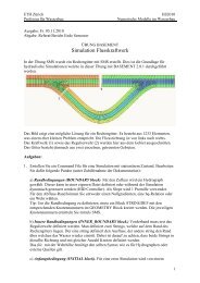
Fig. 1: Definition sketch 

For the control volume illustrated in figure 1, assuming the mass density ρ is constant, it 

can be written: 

VAW ETH Zürich R I - 1.1-1 

Version 9/28/2006


dV 

dt 

d 

= + − − − 

dt 

x2 

∫ Ad x Qout Qin ql 

( x 

x 

2 

x1) 0 

1 

where: A [m 2 ] wetted cross section area 

Q [m 3 /s] discharge 

q [m 2 /s] lateral discharge per meter of length 

l 

V [m 3 ] volume 

x [m] distance 

t [s] time 


= (RI-1.1) 

Applying Leibnitz’s rule and the mean value theorem: 

x2 

x2 

∂A 

∂A 

Ax d d x ( x2 x1 

t∫ = 

x ∫ = − ), 

1 ∂t ∂x 

x1 

d 

d 

and then dividing by ( x2 − x1) 


Q 

out 

− Q 

in 

( x − x1) 

2 

∂Q 

= 

∂x 

the divergent form of the continuity equation is obtained: 

∂A ∂Q + − ql = 0 

∂t 

∂x 

, 

(RI-1.2) 

1.1.2.2 Momentum Conservation 

With the momentum 

dM 

dt 

= m a =∑ F 

where: M 

p = mu 

[kg m/s] momentum 

m [kg] mass 

u [m/s] velocity 

a [m/s 2 ] acceleration 

F [N] force 

and according to Newton’s second law of motion 

Making use of the Reynolds transport theorem (Chaudhry 1993) and referring to the control 

volume in Fig. 1 

dM 

dt 

x2 

d 

∑ F u Adx u2 Au 

2 2 

u1 Au 

1 1 

ux 

ql 

x2 x1 

dt 

∫ ρ ρ ρ ρ ( ) (RI-1.3) 

x1 

= = + − − − 

is obtained, where: 

u 

x 

[m/s] velocity in x direction (direction of flow) of lateral source 

ρ [kg/m 3 ] mass density 

Further simplification is achieved by applying Leibnitz’s rule and writing Q = Au and 

Q/ 

A= 

u resulting in: 

R I - 1.1-2 


Version 9/28/2006



x2 

2 2 

∂Q Q Q 

∑ F= ∫ ρ d x + ρ −ρ −uxρql( 

x2 − x1) 

(RI-1.4) 

∂t A A 

x1 

out 

in 

Application of the mean value theorem: 

and division by ( x2 x1) 

ρ − and with 

x2 

∫ 

x1 

Q Q 

ρ ∂ dx = ∂ ( x2 −x1) 

∂t 

∂x 

⎛ ⎞ ∂ ⎛ ⎞ 

2 2 

Q Q 1 Q 2 

− = 

⎜ A A ⎟ ⎜ ⎟ 

( x2 −x1) 

∂x A 

out in 

⎝ ⎠ 

⎝ 

leads to: 

⎠ 

∑ 2 

F ∂Q 

∂ ⎛Q 

⎞ 

= + ⎜ ⎟−qu 

l x 

x2 x1 

t x A 

(RI-1.5) 

ρ( − ) ∂ ∂ ⎝ ⎠ 

For the determination of 

considered: 

∑F 

the following forces acting on the control volume have to be 

- pressure force upstream and downstream: F1 = ρgA1h1 and F2 

= ρgA 

2 

h 2 

- weight of water in x-direction: 

x2 

F3 

= ρg∫ 

ASBdx 

x2 

QQ 

- frictional force: F4 

= ρg∫ AS 

f 

dx 

, where S 

f 

= 

2 

K 

x1 

x1 

S 

f 

[-] friction slope 

K [m 3 /s] conveyance factor 

g [m/s 2 ] gravity 

k 

st 

[m 1/3 /s] Strickler factor 

R [m] hydraulic radius 

K = k AR 

st 

2 3 

Introducing the sum of these forces in equation (RI-1.5) and applying the mean value 

theorem: 

x2 

∫ AS ( 

B 

− Sf)d x= AS ( 

B 

−Sf)( 

x2 −x1) 

x1 

the momentum equation in the conservation form is obtained: 

⎛ ⎞ 

⎜ ⎟ g ( ) g ( ) 

∂t ∂x⎝ 

A ⎠ ∂x 

2 

∂Q 

∂ Q 

∂ 

+ − ux =− Ah + A SB − 

f 

S (RI-1.6) 


Version 9/28/2006



As 

⎡ 

( Ah) 

A( h h) 1 B( ) 2 ⎤ 

Δ = 

⎢ 

+Δ − Δ − A 

⎣ 

2 ⎥ 

h 

⎦ 

and furthermore neglecting higher order terms and letting 

∂ ∂ ∂ ∂h 

∂h 

Δh→ 0, ( Ah) 

= Aand (g Ah) = g ( Ah) = gA ∂h ∂x ∂h ∂x 

∂ . x 

Equation (RI-1.6) becomes: 

2 

∂Q ∂ ⎛Q ⎞ ∂h 

+ ⎜ ⎟+ g A −gA( S −S ) −qu 

∂t ∂x⎝ 

A ⎠ ∂x 

B f l x 

= 0 

(RI-1.7) 

h 

As and SB 

are unknown for irregular cross sections, they are eliminated from equation 

(RI-1.7) by the following transformation: 

∂h 

∂zS ∂zB 

∂zS 

h= zS 

− zB 

and = − = + S B 

∂x ∂x ∂x ∂x 

Insertion into equation (RI-1.7) results in: 

2 

∂Q ∂ ⎛Q ⎞ ∂z 

+ ⎜ ⎟+ gA + gASf −qu 

l x 

∂t ∂x⎝ 

A ⎠ ∂x 

= 0 

(RI-1.8) 

If only the cross sectional area where the water actually flows and therefore contributes to 

the momentum balance shall be used, and introducing a factor β accounting for the 

velocity distribution in the cross section (Cunge, Holly et al. 1980), equation (RI-1.9) is 

obtained: 

∂ ∂ ⎛ ⎞ ∂ 

∂ ∂ ⎝ ⎠ ∂ 

2 

Q Q z 

+ ⎜β 

⎟+ gAred + gAred S 

f 

−qlux 

t x Ared 

x 

0 

= (RI-1.9) 

where A [m 2 

] is the reduced area, i.e. the part of the cross section area where water 

flows. 

red 

R I - 1.1-4 


Version 9/28/2006



1.1.3 Source Terms 

With the given formulation of the flow equation there are 4 source terms: 

For the continuity equation: 

• The lateral in- or outflow ql 

For the momentum equation: 

• The bed slope 

∂zS 

W = gA 

(RI-1.10) 

∂ x 

• The bottom friction: 

Fr = gA 

red 

S f 

(RI-1.11) 

• The influence of lateral in- or outflow: 

qu 

l 

x 

(RI-1.12) 

However, in this work, the influence of the lateral inflow on the momentum equation is 

neglected. 

1.1.4 Closure Conditions: Determination of the friction Slope S 

f 

The relation between the friction slope and the bottom shear stress is: 

τ 

B 

gRS f 

ρ = (RI-1.13) 

As the unit of τ 

B 

/ ρ is the square of a velocity, a shear stress velocity can be defined as: 

u 

τ 

ρ 

B 

* 

= . (RI-1.14) 

The velocity in the channel is proportional to the shear flow velocity and thus: 

u = c gRS 

(RI-1.15) 

f 

where 

f 

c 

f 

is the Chézy coefficient. 

If u is replaced by Q/ 

A: 

Q c 

f 

g R S 

f 

A = (RI-1.16) 

results, with 


Version 9/28/2006



S 

f 

QQ 

= . (RI-1.17) 

gA cR 

2 2 

f 

Introducing the conveyance K : 

Q 

K = = Acf 

R g 

(RI-1.18) 

S 

f 

S 

f 

QQ 

= (RI-1.19) 

2 

K 

If the Strickler coefficient is used as friction parameter the coefficient 

follows: 

c 

f 

is calculated as 

Strickler: 

1 6 

kstrR 

c 

f 

= (RI-1.20) 

g 

Otherwise the following approaches are implemented: 

Chézy: 

c 

f 

⎛12R 

⎞ 

= 5.75log ⎜ ⎟ (RI-1.21) 

⎝ k ⎠ 

s 

Darcy-Weissbach: 

c f 

8 

= with 

f 

f 

0.24 

= 

⎛12R 

⎞ 

log ⎜ ⎟ 

⎝ ks 

⎠ 

(RI-1.22) 

If it is assumed that the friction depends on the grain size of the bottom: 

k 

str 


ks 

factor 

= default value of factor = 21.1 (RI-1.23) 

6 

d 

90 

90 

= 2d 

(RI-1.24) 

R I - 1.1-6 


Version 9/28/2006



1.1.5 Boundary Conditions 

At the upper und lower end of the channel it is necessary to know the influence of the 

region outside on the flow within the computational domain. The influenced area depends 

on the propagation velocity of a perturbation. The propagation velocity in standing water is 

c= gh (RI-1.25) 

If a one dimensional flow is considered this propagation takes place in two directions: 

upstream ( −c 

) and downstream ( + c ). These velocities must then be added to the flow 

velocities in the channel, giving the upstream (C − 

) and downstream (C + 

) characteristics: 

C 

C 

− 

+ 

dx 

= = u−c dt 

(RI-1.26) 

dx 

= = u+c dt 

(RI-1.27) 

With these functions it is possible to determine which region is influenced by a perturbation 

and which region influences a given point after a given time. 

In particular it can be said that if c

upstream direction, thus the condition in a point cannot influence any upstream point, and a 

point cannot receive any information from downstream. This is the case for a supercritical 

flow. 

In contrast, if c > u, which is the case for sub-critical flow, the information spreads in both 

directions, upstream and downstream. This fact substantiates the necessity and usefulness 

of information at the boundaries. As there are two equations to solve, two variables are 

needed for the solution. 

If the flow conditions are sub-critical, the flow is influenced from downstream. Thus at the 

inflow boundary one condition can be taken from the flow region itself and only one 

additional boundary condition is needed. At the outflow boundary, the flow is influenced 

from outside and so one boundary condition is needed. 

If the flow is supercritical, no information arrives from downstream. Therefore, two 

boundary conditions are needed at the inflow end. In contrast, as it cannot influence the 

flow within the computational domain, it is not useful to have a boundary condition at the 

downstream end. 

Number of boundary conditions 

Flow type Inflow Outflow 

Sub critical flow ( Fr < 1) 1 2 

Supercritical flow ( Fr > 1 ) 

1 0 

Tab. 1: Number of needed boundary conditions 


Version 9/28/2006



At the inflow boundary the given value is usually Q . If the flow is supercritical the second 

variable A is determined by a flow resistance law (slope is needed!). 

At the outflow boundary there are several possibilities to provide the necessary information 

at the boundary: 

- determine an out flowing discharge by a weir or a gate; 

- set the water surface elevation as a function of time; 

- set the water surface elevation as a function of the discharge (rating curve). 

R I - 1.1-8 


Version 9/28/2006



1.2 Shallow Water Equations 


Mathematical models of the so-called shallow water type govern a wide variety of physical 

phenomena. An important class of problems of practical interest involves water flows with a 

free surface under the influence of gravity. It includes: 

- Tides in oceans 

- Flood waves in rivers 

- Dam break waves 

A key assumption made in derivation of the approximate shallow water theory concerns the 

pressure distribution. Supposing that the vertical velocity acceleration of water particles is 

negligible, a hydrostatic pressure distribution can be assumed. This eventually allows for a 

integration over the flow depth, which results in a non-linear initial value problem, namely 

the shallow water equations. They form a time-dependent two-dimensional system of nonlinear 

partial differential equations of hyperbolic type. 

There are two approaches for the derivation of shallow water equations: 

- Integrating the three-dimensional system of Navier-Stokes equations over the 

depth 

- Direct approach by considering a three-dimensional control volume element of 

fluid 

Note, that for reason of simplicity, the shallow water equations will from here on be 

abbreviated as SWE. 

Using the first method and imposing the following boundary conditions: 

1) At the top of water surface: 

Kinetic boundary condition: 

∂zs 

∂zs 

∂z wS = + uS + v s 

S 

∂t 

∂x 

∂y 

(RI-1.28) 

Dynamic boundary condition: 

( ) 

τ = τ , τ and P =P 

(RI-1.29) 

Sx Sy atm 


Version 9/28/2006



2) At the bottom of water body: 

Kinetic boundary condition: 

∂zB 

∂zB 

wB = uB + vB 

∂x 

∂y 

(RI-1.30) 

The set of SWE can be derived in the form: 

( uh) ( vh) 

∂ ζ ∂ ∂ 

+ + 

∂t ∂x ∂y 

= 0 

(RI-1.31) 

∂u ∂u ∂u ⎛∂Z B 

∂h⎞ 

1 τ 

+ u + v + g 

Bx 

⎜ + ⎟=− 

∂t ∂x ∂y ⎝ ∂x ∂x⎠ 

h ρ 

∂v ∂v ∂v ⎛∂Z B 

∂h⎞ 

1 τ By 

+ u + v + g⎜ 

+ ⎟=− 

∂t ∂x ∂y ⎝ ∂y ∂y⎠ 

h ρ 

(RI-1.32) 

(RI-1.33) 

where: h [m] water depth 

g [m/s 2 ] gravity acceleration 

P [Pa] pressure 

u [m/s] depth averaged velocity in x direction 

u S 

[m/s] velocity in x direction at water surface; 

u B 

[m/s] velocity in x direction at bottom (usually equal zero) 

v [m/s] depth averaged velocity in y direction 

v S 

[m/s] velocity in y direction at water surface 

v B 

[m/s] velocity in y direction at bottom (usually equal zero) 

w S 

[m/s] velocity in z direction at water surface 

w B 

[m/s] velocity in z direction at bottom (usually equal zero) 

w B 

[m] velocity in z direction at bottom (usually equal zero) 

z B 

[m] bottom elevation 

z 

s 

[m] water surface elevation 

τ 

Sx , 

[N/m 2 ] surface stress in x direction such as wind stress 

τ 

S, 

y 

[N/m 2 ] surface stress in y direction such as wind stress 

τ 

Bx , 

[N/m 2 ] bottom stress in x direction 

τ [N/m 2 ] bottom stress in y direction 

By , 

For brevity, the over bars indicating depth averaged values will be dropped from 

from here on. 

u 

and v 

R I - 1.2-2 


Version 9/28/2006



1.2.2 Conservative Form of SWE 

Various forms of SWE can be distinguished with their primitive variables. The proper choice 

of these variables and the corresponding set of equations plays an extremely important role 

in numerical modelling. It is well known that the conservative form is preferred over the 

non-conservative one if strong changes or discontinuities in a solution are to be expected. In 

flooding and dam break problems, this is usually the case. 

(Bechteler, Nujić et al. 1993) showed that the equation sets in conservative form, with 

( huhvh , , ) as independent and primitive variables produce best results. The conservative 

form can be derived by multiplying the continuity equation with u and v and adding to 

momentum equations in x and y direction respectively. This set of equations can be written 

in the following form: 

( ) 

U +∇⋅ F, 

G + S = 0 

(RI-1.34) 

t 

S 

where U, 

Q and are the vectors of primitive variables, fluxes in the x and y directions 

and sources respectively, given by: 

⎛ζ 

⎞ 

⎜ ⎟ 

U = uh 

⎜vh 

⎟ 

⎝ ⎠ 

⎛ ⎞ ⎛ ⎞ 

⎜ uh ⎟ ⎜ uh ⎟ 

⎜ ⎟ ⎜ ⎟ 

2 1 2 ∂u 

2 1 2 ∂u 

F= ⎜uh+ gh − νh ⎟; 

G = ⎜uh+ gh −νh 

⎟ (RI-1.35) 

⎜ 2 ∂x 

⎟ ⎜ 2 ∂x 

⎟ 

⎜ 

v 

⎟ ⎜ 

v 

⎟ 

⎜ 

∂ 

∂ 

uvh −νh ⎟ ⎜ uvh −νh 

⎟ 

⎝ ∂x 

⎠ ⎝ ∂x 

⎠ 

⎛ 0 

⎜ 

S = ⎜gh S − 

⎜ 

⎜ 

⎝ 

gh S 

( fx 

SBx 

) 

( fy 

− SBy 

) 

⎞ 

⎟ 

⎟ 

⎟ 

⎟ 

⎠ 

where: 

* 

ν is the isotropic eddy viscosity computed as ν = ν0 + cUh 

μ 

. ν 

0 

= base kinematic eddy 

viscosity and c μ 

= dimensionless coefficient. 


Version 9/28/2006



1.2.3 Source Tems 

Eqation (RI-1.36) has two source terms, bed stress ( τ 

B 

= ghS f 

) and bed slope terms 

( ghS B 

). 

The bed stress is the most important physical parameter besides water depth and velocity 

field of a hydro- and morphodynamic model. It causes the turbulence and is responsible for 

sediment transport and has a non-linear effect of retarding the flow. When the effect of 

turbulence grows, the effect of molecular viscosity becomes relatively smaller, while viscous 

boundary layer near a solid boundary becomes thinner and may even appear not to exist. It 

means that the bed stress (friction) is equal to the bed turbulent stress. 

(Prandtl 1942) has obtained the following relation for τ 

B 

with assumption of logarithmic law 

for vertical velocity profile: 

τ 

uz ( ) − uz ( ) 

1 2 

B 

= κ 

log 

2 1 

( z z ) 

where κ = von Karman constant; z = height above bottom. 

(RI-1.37) 

However, bed stress is usually estimated by using an empirical or semi-empirical formula 

since the vertical distribution of velocity cannot be readily obtained. 

In the one dimensional system of equations the term bed stress can be expressed as 

gRS 

f 

, where S 

f 

denotes the energy slope. Assuming that the frictional force in a two 

dimensional unsteady open flow can be estimated by referring to the formulas for one 

dimensional flows in open channel, e.g. by Manning’s Formula, it can be written: 

S 

f 

2 

nuu 

4 3 

= (RI-1.38) 

R 

where u = velocity; n = Manning’s factor; R = hydraulic radius. It can be easily seen that 

the above formula can be approximately generalized to the two dimensional system. In onedimensional 

flows it is not distinguished between bottom and lateral (side wall) friction, 

while in two dimensional flows it is often taken a unit width channel ( R = h). For the two 

dimensional system the Equation (RI-1.38) has the following forms 

fx 

4 4 

2 2 2 3 2 2 2 

; 

fy 

3 

S = n u u + v h S = n v u + v h 

(RI-1.39) 

The bed stress terms need additional closures equation (see chapter 1.2.5) to be 

determined. Here we used the Manning’s formula. 

Bed slope terms represent the gravity forces 

Bx , 

=−∂ 

B 

∂ ; 

By , 

S z x 

S =−∂z ∂ y 

(RI-1.40) 

B 

R I - 1.2-4 


Version 9/28/2006



1.2.4 Boundary Conditions 

SWE provide a model to describe dynamic fluid processes of various natural phenomena 

and find therefore widespread application in science and engineering. Solving SWE needs 

the appropriate boundary conditions like any other partial differential equations. In particular, 

the issue of which kind of boundary conditions are allowed is still not completely understood 

(Agoshkov, Quarteroni et al. 1994). However several sets of boundary conditions of physical 

interest that are admissible from the mathematical viewpoint will be discussed here. 

The physical boundaries can be divided into two sets: one closed ( Γ 

c 

), the other open ( Γ 

o 

) 

(Fig. 2). The former generally expresses that no mass can flow through the boundary. The 

latter is an imaginary fluid-fluid boundary and includes two different inflow and outflow 

types. 

1.2.4.1 Closed Boundary 

The following relations are often described on the closed boundary, say 

∂u 

ρun 

⋅ = 0; = 0 

∂n 

where n [m] the normal (directed outward) unit vector on 

u [m/s] velocity vector = ( uv , ) 

Γ 

c 

Γ 

c 

: 

(RI-1.41) 

Fig. 2: Computational Domain and Boundaries 

1.2.4.2 Open Boundary 

The number of boundaries of a partial differential equations system depends on the type of 

the system. From the mathematical point of view, the SWE establish a quasi-linear 

hyperbolic differential equations system. If the temporal derivatives vanish, the system is 

elliptical for Fr 

≤1.0 

and hyperbolical for Fr 

≥1.0 

, where Fr 

is Froude number. 

On the open boundary ( Γ o 

) the two types inflow and outflow can be respectively 

distinguished as follows: 

Γ = ( x ∈Γ ; 0 

un ⋅ < ) 

in 

0 (RI-1.42) 


Version 9/28/2006



Γ = ( x∈Γ ; 0 

⋅ > 

out 

0) 

un (RI-1.43) 

Based on the behaviour of the system of equations, the theoretical number of open 

boundary conditions is listed in Tab. 2 (Agoshkov, Quarteroni et al. 1994) (Beffa 1994): 

Number of boundary conditions 

Flow type Inflow Outflow 

Sub critical flow ( Fr < 1) 2 1 

Supercritical flow ( Fr > 1 ) 

3 0 

Tab. 2: The Correct Number of Boundary Conditions in SWE 

However in practical application of boundary conditions, the number of the implemented 

conditions is often higher or lower than the theoretical criteria (Nujić 1998). 

1.2.5 Closure Conditions 

1.2.5.1 Turbulence Closure 

The turbulent shear stresses can be quantified in accordance with the Boussinesq eddyviscosity 

concept, which can be expressed as 

τxx 2 ρν ∂u t 

, τ 

yy 

2 ρν ∂v t 

, τ u v 

xy 

ρν ⎛∂ 

∂ 

= = = ⎞ 

t ⎜ + ⎟ 

∂x ∂y ⎝∂y 

∂x⎠ 

(RI-1.44) 

If the flow is dominated by the friction forces, the turbulent kinematic viscosity is 

ν = κuh 

with the friction velocity u* 

= τ ρ . 

t 

* 

6 

1.2.5.2 Bed Stress 

The bed shear stresses are related to the depth–averaged velocities by the quadratic friction 

law 

u u u v 

τ ρ τ ρ 

bx 

= , 

2 by 

= 

2 

cf 

cf 

= u + v 

(RI-1.45) 

2 2 

in which u is the magnitude of the velocity vector. The friction coefficient c 

f 

can be determined by any friction law. 

R I - 1.2-6 


Version 9/28/2006



2 Sediment and Pollutant Transport 

2.1 Suspended Sediment and Pollutant Transport 

2.1.1 Addvection-Diffusion-Equation 

According to the number of pollutant species or grain size classes, ng advection-diffusion 

equations for transport of the suspended material are provided as follows: 

∂ ∂ ⎛ ∂Cg 

⎞ ∂ ⎛ ∂Cg 

⎞ 

Ch 

g 

+ ⎜Cq g 

−hΓ ⎟+ ⎜Cr g 

−hΓ ⎟− Sg 

= 0 forg= 

1,..., ng 

∂t ∂x⎝ ∂x ⎠ ∂y⎝ ∂y 

⎠ 

where 

C 

g 

is the concentration of each grain size class and Γ is the eddy diffusivity. 

(RI-2.1) 


Version 9/28/2006



This page has been intentionally left blank. 

R I - 2.1-2 


Version 9/28/2006



2.2 Bed Load Transport 


The bed load flux in x direction is composed of three parts (an analogous relation exists in y 

direction): 

q = q + q + q 

Bg , x Bg, xx Bg, xy Bg, 

gravx 

q q B , xy 

(RI-2.2) 

where 

B 

= bed load transport due to flow in x direction, = lateral transport due to 

g , xx 

g 

bed load transport in y direction and q 

Bg 

, grav 

= pure gravity induced transport (e.g. due to 

x 

collapse of a side slope). 

2.2.2 Bed Material Sorting 

For each fractio g mass conservation equation can be written, the so called “bed-material 

sorting equation”: 

∂ ∂q 

∂qBg y 

1− p 

g 

⋅ hm + + + Sg −Sfg 

− YX = 0 for g = 1,..., ng 

∂t ∂x ∂y 

Bg, x 

, 

( ) ( β ) 

(RI-2.3) 

where p = porosity of bed material (assumed to be constant), ( qBg, x, 

qBg, 

y) = 

components of total bed load flux per unit width, Sf 

g 

= flux through the bottom of the 

active layer due to its movement and Sl 

g 

= source term to specify a local input or output of 

material (e.g. rock fall, dredging). 

2.2.3 Mass Conservation 

Finally, the global bed material conservation equation is obtained by adding up the masses 

of all sediment material layers between the bed surface and a reference level for all 

fractions (Exner-equation) directly resulting in the elevation change of the actual bed level: 

ng 

B 

Bg, x Bg, 

y 

− 

B 

+ ∑ + + S − 

t ⎜ 

g 

Sl 

g 

= 0 

∂ g = 1 ∂x ∂y 

⎟ 

( 1 p ) 

∂z 

⎛∂q 

⎝ 

∂q 

⎞ 

⎠ 

(RI-2.4) 


Version 9/28/2006



2.2.4 Bottom Shear stress and Motion Threshold 

The critical shear stress τ θ ( ρ ρ) 

= − 

g 

is the threshold for the initiation of motion 

of the grain class g and is derived from the according Shields parameter θ 

cr 

, which is a 

* 

function of the shear Reynolds number Re see (Shields 1936). Meyer-Peter and Müller 

(1948) proposed a constant Shields parameter of 0.047 for the fully turbulent area 

* 3 * 

* 

( Re > 10 ). For smaller values of Re , the Shields parameter θ 

cr 

= f ( D ) is evaluated as 

* 

function of the dimensionless grain diameter D according to (Van Rijn 1984) (see Fig. 3). 

Bcr 

cr s 

gd 

Fig. 3: Determination of critical shear stress for a given grain diameter 

R I - 2.2-2 


Version 9/28/2006



2.2.5 Closures for Bed Load Transport 

Bed load transport is evaluated as follows 

q 

, 

= β q ( ξ ) ⋅e (RI-2.5) 

Bg 

x g Bg 

g x 

Approaches for the bed load discharge q ( ξ ) with or without the consideration of the 

hiding factor ξ are discussed in following section. 

g 

Bg 

g 

2.2.5.1 Transport Laws 

The specific bed load discharge 

equation. 

th 

q of the grain class has to be evaluated by a suitable 

B g 

g 

2.2.5.1.1 Meyer-Peter and Müller (MPM) 

The (Meyer-Peter and Müller 1948) formula can be written as follows: 

q B g 

3 2 

B 

−τB , 1 

cr g 

⎛τ 

⎞ ⎛ ⎞ 

= ⎜ ⎟ ⎜ ⎟ 

⎝ 0.25 ρ ⎠ ⎝( s−1) 

g ⎠ 

Herein, τ 

B 

is the shear stress induced by the flow and 

coefficient. 

(RI-2.6) 

s = ρs 

ρ the sediment density 

2.2.5.1.2 Parker 

(Parker 1990) has extended his empirical substrate-based bedload relation for gravel 

mixtures (Parker, Klingeman et al. 1982), which was developed solely with reference to field 

data and suitable for near equilibrium mobile bed conditions, into a surfaced-based relation. 

The new relation is proper for the nonequilibrium processes. 

Based on the fact that the rough equality of bedlaod and substrate size distribution is 

attained by means of selective transport of surface material and the surface material is the 

source for bedlaod, Parker has developed the new relation based on the surface material. 

An important assumption in deriving the new relation is suspension cutoff size. He suppose 

that during flow conditions at which significant amounts of gravel are moved, it is commonly 

(but not universally) found that the sand moves essentially in suspension (1-6 mm). There 

for he has excluded sand from his analysis. In his free access Excel file, he has explicitly 

emphasised that the formula is valid only for the size larger than 2 mm. 

Regarding to the Oak Creek data, the original relation predicted 13% of the bedload as sand. 

For consistency it has to be corrected for the exclusion of sand and finer material. 


Version 9/28/2006



W 

0.00218 G⎡ξωφ 

= ⎣ ⎦ ; * 

Wsi 

( τ ρ) 

* 

si s sg 0 

where 

⎤ 

Rgqbi 

= (RI-2.7) 

3/2 

F 

i 

ξ 

⎛ d 

⎞ 

i 

s 

= ⎜ 

d ⎟ 

g 

⎝ 

⎠ 

−0.0951 

; 

φ 

τ 

* 

sg 

50 * 

τ 

rsg 0 

= ; 

τ 

* 

sg 

τ 

ρRgd g 

= ; 

* 

τ 

rsg 0 

= 0.0386 

σ 

⎡ln 

( d ) 

⎡ 

0( sg 0) 

⎤ 

( φsg 

) 

⎣ ⎦ ; i 

dg 

σ Fi 

⎢ ln ( 2) 

ω = 1+ ω φ −1 

σ 

0 0 

⎤ 

= ∑ ⎢ ⎥ ; 

⎣ ⎥⎦ 

2 

dg 

= e ∑ 

Filn( di) 

ξ 

s 

is a “reduced” hiding function and differs from the one of Einstein. The Einstein hiding 

factor adjusts the mobility of each grain d i in a mixture relative to the value that would be 

realized if the bed were covered with uniform material of size d i . The new function adjusts 

the mobility of each grain d i relative to the d 50 or d g , where d g denotes the surface geometric 

mean size. 

Although the above formulation does not contain a critical shields stress, the reference 

Schields stress τ * rsg 0 

makes up for it, in that transport rates are exceedingly small for 

* * 

τ 

sg 

< τ 

rsg 0 

. Regarding to the fact that parker’s relation is based on field data and field data 

are often in case of low flow rates, the relation calculates low bedload rates (Marti 2006). 

2.2.5.2 Hunziker (MPM-H) 

To map transport processes of mixed sediments and to calculate according bed load 

discharge, corrections or special formulas for graded sediments have to be applied. Besides 

the ability to model grain sorting in the active layer, the exposure of bigger grains to the flow 

and the involved shielding of fine sediments, the so called hiding effect has to be 

considered. 

A special formula for the fractional transport of graded sediments was proposed by 

(Hunziker 1995): 

q 

( ) 3 2 

⎤ 

= 5 β ⎡ 

⎣ 

ξ θ −θ 

⎦ 

( s−1)gd 

' 3 

Bg 

g g dms cdms ms 

) 

(RI-2.8) 

' 

The additional shear stress ( θdms 

−θcdms 

regarding the mean grain size of the bed surface 

material is corrected by a corresponding hiding factor: 

ξ 

−α 

⎛ d 

g ⎞ 

g 

= ⎜ ⎟ 

dms 

⎝ 

⎠ 

(RI-2.9) 

where dms 

denotes the mean diameter of the active layer and α is an empirical parameter 

which depends on the dimensionless shear stress of the mixture (see also (Hunziker and 

Jaeggi 2002)). 

R I - 2.2-4 


Version 9/28/2006



2.2.5.3 Günter’s two grains model 

(Günter 1971) suggested a two grains model, in order to be able to consider the armoured 

layer forming in case of the simulation with one grain size. Based on his formulation, the 

upper limit of the discharge of the armoured layer (Q D ) can be calculated, for which the 

armoured layer resists it. If the discharge is smaller than Q D , then no material will be eroded 

from the bed, but the input bedload from the upstream can be transported into the 

downstream. 

Using the formulation of Günter one obtains 

RSf 

d 

θ ⎛ ⎞ 

s− d ⎝ d ⎠ 

( 1) 

90 

> 

c ⎜ ⎟ 

m 

m 

0.67 

Where R denotes hydraulic radius, S f is energy slope, d m is grain size, d 90 is armoured layer 

grain size and θ 

c 

denotes the critical Shield’s parameter for the grain size (d m ). 

(Hunziker and Jaeggi 1988) analysed Günter’s relation and concluded that it should not be 

always used. If there are aggradations on an armoured layer, then it should be possible to 

transport the material. In this case, the elevation of the armoured layer has to be saved and 

compared with the new bed elevation. 

2.2.6 Source Terms 

The exchange of sediment particles between the active layer and the underlying sublayer 

made up of material with size fractions β is expressed by the source term: 

g 

S g 

∂ 

Sfg 

=−(1 −p) (( zB 

−hm) β ) 

∂t 

with β = β in case of aggradation (active layer is rising) and β = β Sg 

in case of erosion. 

(RI-2.10) 


Version 9/28/2006




R I - 2.2-6 


Version 9/28/2006



2.3 Lateral Transport 

The lateral transport occurring on a transverse bed slope is determined according to the 

approach of (Ikeda 1982): 

q 

⎛ 

τ 

Bcr 

, g 

B , 

1.5 

g xy 

= Sx ⎜ 

B yy 

τ 

Bx , ⎟ 

g, 

⎝ 

⎞ 

⎠ 

q (RI-2.11) 

q 

where: S 

x 

= bed slope in x direction, 

B , 

= bed load of fraction in y direction and 

g yy 

g 

τ = critical shear stress of the individual grain class. 

Bcr 

, g 


Version 9/28/2006




R I - 2.3-2 


Version 9/28/2006



References 

Agoshkov, V. I., A. Quarteroni, et al. (1994). "Recent Developments in the Numerical- 

Simulation of Shallow-Water Equations .1. Boundary-Conditions." Applied Numerical 

Mathematics 15(2): 175-200. 

Bechteler, W., M. Nujić, et al. (1993). Program Package “FLOODSIM“ and ist Application. 

Beffa, C. J. (1994). Praktische Lösung der tiefengemittelten Flchwassergleichungen. 

Versuchsanstalt für Wasserbau,Hydrologie und Glaziologie (VAW). Zürich, ETH 

Zürich. 

Chaudhry, M. H. (1993). Open-Channel Flow. Englewood Cliffs, New Jersey, Prentice Hall. 

Cunge, J. A., F. M. J. Holly, et al. (1980). Practical aspects of computational river hydraulics. 

London, Pitman. 

Günter, A. (1971). Die kritische mittlere Sohlenschubspannung bei Geschiebemischung 

unter Berücksichtigung der Deckscichtbildung und der turbulenzbedingten 

Sohlenschubspannungsschwankungen. Versuchsanstalt für Wasserbau,Hydrologie 

und Glaziologie (VAW). Zürich, ETH Zürich. 

Hunziker, R. P. (1995). Fraktionsweiser Geschiebetransport. Versuchsanstalt für 

Wasserbau,Hydrologie und Glaziologie (VAW). Zürich, ETH Zürich. 

Hunziker, R. P. and M. N. R. Jaeggi (1988). Numerische Simulation des Geschiebehaushalts 

der Emme. Interprävent, Graz. 

Hunziker, R. P. and M. N. R. Jaeggi (2002). "Grain sorting processes." Journal of Hydraulic 

Engineering-Asce 128(12): 1060-1068. 

Ikeda, S. (1982). "Lateral Bed-Load Transport on Side Slopes." Journal of the Hydraulics 

Division-Asce 108(11): 1369-1373. 

Marti, C. (2006). Morphologie von verzweigten Gerinnen Ansätze zur Abfluss-, 

Geschiebetransport und Kolktiefenberechnung. Versuchsanstalt für 

Wasserbau,Hydrologie und Glaziologie (VAW). Zürich, ETH Zürich. 

Meyer-Peter, E. and R. Müller (1948). Formulas for Bed-Load Transport. 2nd Meeting IAHR, 

Stockholm, Sweden, IAHR. 

Nujić, M. (1998). Praktischer Einsatz eines hochgenauen Verfahrens für die Berechnung von 

tiefengemittelten Strömungen. Institut für Wasserwesen. München, Universität der 

Bundeswehr München. 

Parker, G. (1990). "Surface-based bedload transport relation for gravel rivers." Journal of 

Hydraulic Reasearch 28(4): 417-436. 

Parker, G., P. C. Klingeman, et al. (1982). "Bedlaod and size distribution in paved gravel-bed 

streams." Journal of Hydraulic Division, ASCE(108): 544-571. 

Prandtl, L. (1942). "Comments on the theory of free turbulence." Zeitschrift Fur Angewandte 

Mathematik Und Mechanik 22: 241-243. 

Shields, A. (1936). Anwendungen der Ähnlichkeitsmechanik und der Turbulenzforschung auf 

die Geschiebebewegungen. Preussische Versuchsanstalt für Wasserbau und 

Schiffbau. Berlin, Deutschland. 

Van Rijn, L. C. (1984). "Sediment Transport, Part II: Suspended Load Transport." Journal of 

Hydraulic Engineering, ASCE 110(11). 


Version 9/28/2006 

R I - References


NUMERICS KERNEL 


1 General View ....................................................................................... 1-1 

2 Methods for Solving the Flow Equations 

2.1 Fundamentals .................................................................................................... 2.1-1 

2.1.1 Finite Volume Method.................................................................................. 2.1-1 

2.1.2 The Riemann Problem.................................................................................. 2.1-3 

2.1.3 Riemann Solvers........................................................................................... 2.1-4 

2.2 Saint-Venant Equations .................................................................................... 2.2-1 

2.2.1 Spatial Discretization .................................................................................... 2.2-1 

2.2.2 Discrete Form of Equations.......................................................................... 2.2-1 

2.2.3 Discretisation of Source Terms .................................................................... 2.2-2 

2.2.4 Discretisation of Boundary conditions.......................................................... 2.2-7 

2.2.5 Solution Procedure ....................................................................................... 2.2-9 

2.3 Shallow Water Equations ................................................................................. 2.3-1 


2.3.2 Discretization of Source Terms .................................................................... 2.3-4 

2.3.3 Discretization of Boundary Conditions ......................................................... 2.3-8 

2.3.4 Solution Procedure ..................................................................................... 2.3-12 

3 Solution of Sediment Transport Equations 

3.1 General Vertical Partition ................................................................................. 3.1-1 

3.1.1 Vertical Discretization ................................................................................... 3.1-1 

3.1.2 Determination of Layer Thickness................................................................ 3.1-2 

3.2 One Dimensional Sediment Transport............................................................ 3.2-1 

3.2.1 Spatial Discretisation .................................................................................... 3.2-1 

3.2.2 Discrete form of equations........................................................................... 3.2-2 


3.3 Two Dimensional Sediment Transport ........................................................... 3.3-1 

3.3.1 Spatial Discretization .................................................................................... 3.3-1 



4 Time Discretization and Stability Issues 

4.1 Explicit Schemes................................................................................................ 4.1-1 

4.1.1 Euler First Order ........................................................................................... 4.1-1 

4.2 Determination of Time Step Size..................................................................... 4.2-1 

4.2.1 Hydrodynamic............................................................................................... 4.2-1 

4.2.2 Sediment Transport ...................................................................................... 4.2-1 


Version 9/26/2006 

R II - i




Fig. 1: Triangular Finite Elements of a Two-Dimensional Domain..............................................2.1-1 

Fig. 2: Two-Dimensional Finite Volume Mesh: (a) Cell Centered mesh (b) Cell Vertex mesh.....2.1-2 

Fig. 3: Initial Data for Riemann Problem .....................................................................................2.1-3 

Fig. 4: Possible Wave Patterns in the Solution of Riemann Problem (5-5)...................................2.1-4 

Fig. 5: Piecewise constant data of Godunov upwind method ........................................................2.1-5 

Fig. 6: Definition sketch.................................................................................................................2.2-1 

Fig. 7: Simple cross section ...........................................................................................................2.2-4 

Fig. 8: Conveyance computation of a channel with a flat zone .....................................................2.2-4 

Fig. 9: Cross section with flood plains and main channel.............................................................2.2-5 

Fig. 10: Cross section with definition of a bed ................................................................................2.2-5 

Fig. 11: Cross section with flood plains and definition of a bed bottom .........................................2.2-6 

Fig. 12: Geometry of a Computational Cell Ω i 

in FV ...................................................................2.3-2 

Fig. 13: A Triangular Cell ...............................................................................................................2.3-5 

Fig. 14: Water volume over a cell....................................................................................................2.3-6 

Fig. 15: Partially wet cell ................................................................................................................2.3-7 

Fig. 16: Flow over a weir ..............................................................................................................2.3-10 

Fig. 17: Outlet cross section with a weir .......................................................................................2.3-10 

Fig. 18: Schematic representation of a mesh with dry, partial wet and wet elements ...................2.3-11 

Fig. 19: Wetting process of a element............................................................................................2.3-12 

Fig. 20: The logical flow of data through BASEplane...................................................................2.3-13 

Fig. 21: Data flow through the hydrodynamic routine ..................................................................2.3-14 

Fig. 22: Data flow through the morphodynmic routine .................................................................2.3-14 

Fig. 23: Vertical discretization of a computational cell ..................................................................3.1-1 

Fig. 24: Soil discretization in a cross section ..................................................................................3.2-1 

Fig. 25: Effect of bed load on cross section geometry .....................................................................3.2-2 

Fig. 26: Distribution of sediment area change over the cross section.............................................3.2-7 

Fig. 27: Uncoupled asynchronous solution procedure consisting of sequential steps.....................3.3-3 

Fig. 28: Composition of the given overall calculation time step 

Δ tseq 

...........................................3.3-3 

R II - ii 


Version 9/26/2006



II 


1 General View 

There is great improvement in the development of numerical models for free surface flows 

and sediment movement in the last decade. The presented number of publications about 

these subjects proves this clearly. The SWE and the sediment flow equation are a nonlinear, 

coupled partial differential equations system. A unique analytical solution is only possible for 

idealised and simple conditions. For practical cases, it is required to implement the 

numerical methods. A numerical solution arises from the discretization of the equations. 

There are different methods to discretize the equations such as: 

- Finite difference………….(FD) 

- Finite volume…………….(FV) 

- Finite element…………….(FE) 

- Characteristic Method……(CM) 

It is normally distinguished between temporal and spatial discretization of continuum 

equations. The latter can be undertaken on different forms of grids such as Cartesian, nonorthogonal, 

structured and unstructured, while the former is usually done by a FD scheme in 

time direction, which can be explicit or implicit. The explicit method is usually used for 

strong unsteady flows. 

In FD methods the partial derivations of equations are approximated by using Taylor series. 

This method is particularly appropriate for an equidistant Cartesian mesh. 

In FV methods; the partial derivations of equations are not directly approximated like in FD 

methods. Instead of that, the equations are integrated over a volume, which is defined by 

nodes of grids on the mesh. The volume integral terms will be replaced by surface integrals 

using the Gauss formula. These surface integrals define the convective and diffusive fluxes 

through the surfaces. Due to the integration over the volume, the method is fully 

conservative. This is an important property of FV methods. It is known that in order to 

simulate discontinuous transition phenomena such as flood propagation, one must use 

conservative numerical methods. In fact, 40 years ago Lax and Wendroff proved 

mathematically that conservative numerical methods, if convergent, do converge to the 

correct solution of the equations. More recently, Hou and LeFloch proved a complementary 

theorem, which says that if a non-conservative method is used, then the wrong solution will 

be computed, if this contains a discontinuity such as a shock wave (Toro 2001). 

The FE methods originated from the structural analysis field as a result of many years of 

research, mainly between 1940 and 1960. In this method the problem domain is ideally 

subdivided into a collection of small regions, of finite dimensions, called finite elements. The 

elements have either a triangular or a quadrilateral form (Fig. 1) and can be rectilinear or 

VAW ETH Zürich R II - 1-1 

Version 9/26/2006



curved. After subdivision of the domain, the solution of discrete problem is assumed to have 

a prescribed form. This representation of the solution is strongly linked to the geometric 

division of sub domains and characterized by the prescribed nodal values of the mesh. 

These prescribed nodal values must be determined in such way that the partial differential 

equations are satisfied. The errors of the assumed prescribed solution are computed over 

each element and then the error must be minimised over the whole system. One way to do 

this is to multiply the error with some weighting function ω ( x, 

y) 

, integrate over the region 

and require that this weighted-average error is zero. The finite volume method has been 

used in this study; therefore it is explained in more detailed. 

In this chapter it will be reviewed how the governing equations comprising the SWE and the 

bed-updating equation, can be numerically approximated with accuracy. The first section 

studies the fundamentals of the applied methods, namely the finite volume method and 

subsequently the hydro- and morphodynamic models are discussed. In section on the 

hydrodynamic model, the numerical approximate formulation of the SWE, the flux 

estimation based on the Riemann problem and solver and related problems such as 

boundary conditions will be analyzed. In the section on morphodynamics, the numerical 

detemination of the bed stress and the numerical treatment of bed slope stability will be 

discussed as well as numerical approximation of the bed-updating equation. 

R II - 1-2 


Version 9/26/2006



2 Methods for Solving the Flow Equations 

2.1 Fundamentals 

2.1.1 Finite Volume Method 

The basic laws of fluid dynamics and sediment flow are conservation equations; they are 

statements that express the conservation of mass, momentum and energy in a volume 

enclosed by a surface. Conversion of these laws into partial differential equations requires 

sufficient regularity of the solutions. 

Fig. 1: Triangular Finite Elements of a Two-Dimensional Domain 

This condition of regularity cannot always undoubtedly be guaranteed. The case of occurring 

of discontinuities is a situation where an accurate representation of the conservation laws is 

important in a numerical method. In other words, it is extremely important that these 

conservation equations are accurately represented in their integral form. The most natural 

method to achieve this is obviously to discretize the integral form of the equations and not 

the differential form. This is the basis of the finite volume (FV) method. Actually the finite 

volume method is in fact in the classification of the weighted residual method (FE) and 

hence it is conceptually different from the finite difference method. The weighted function 

is chosen equal unity in the finite volume method. 

In this method, the flow field or domain is subdivided, as in the finite element method, into 

a set of non-overlapping cells that cover the whole domain on which the equations are 

applied. On each cell the conservation laws are applied to determine the flow variables in 

some discrete points of the cells, called nodes, which are at typical locations of the cells 

such as cell centres (cell centred mesh) or cell-vertices (cell vertex mesh) (Fig. 2). 

Obviously, there is basically considerable freedom in the choice of the cell shapes. They can 

be triangular, quadrilateral etc. and generate a structured or an unstructured mesh. Due to 

this unstructured form ability, very complex geometries can be handled with ease. This is 

clearly an important advantage of the method. Additionally the solution on the cell is not 

VAW ETH Zürich R II - 2.1-1 

Version 9/26/2006



strongly linked to the geometric representation of the domain. This is another important 

advantage of the finite volume method in contrast to the finite element method. 

Fig. 2: Two-Dimensional Finite Volume Mesh: (a) Cell Centered mesh (b) Cell Vertex mesh 

R II - 2.1-2 


Version 9/26/2006



2.1.2 The Riemann Problem 

Formally, the Riemann problem is defined as an initial-value problem (IVP): 

( ) 

Ut 

+ Fx 

U = 0 ⎫ 

⎪ 

⎧UL 

∀ x < 0⎬ 

U ( x,0) 

= ⎨ 

R 

∀ x > 0 

⎪ 

⎩U 

⎭ 

(RII-2.1) 

Here equations (4-7) and (4-8) are considered for the x-split of SWE. The initial states 

U with 

R 

U = L 

⎛ hL 

⎞ 

⎜ ⎟ 

uh 

L L 

⎜vh 

⎟ 

⎝ L L ⎠ 

; U = R 

⎛ hR 

⎞ 

⎜ ⎟ 

uh 

R R 

⎜vh 

⎟ 

⎝ R R⎠ 

U 

L 

, 

are constant vectors and present conditions to the left of axes x = 0 and to the right x = 0 , 

respectively (Fig. 3). 

U 

U L 

U R 

Fig. 3: Initial Data for Riemann Problem 

There are four possible wave patterns that may occur in the solution of the Riemann 

problem. These are depicted in Fig. 4. In general, the left and right waves are shocks and 

rarefactions, while the middle wave is always a shear wave. A shock is a discontinuity that 

travels with Rankine-Hugoniot shock speed. A rarefaction is a smoothly varying solution 

which is a function of the variable x/t only and exists if the eigenvalues of J =∂F( U)/ 

∂U 

are all real and the eigenvectors are complete. The water depth and the normal velocity are 

both constant across the shear wave, while the tangential velocity component changes 

discontinuously. (See Toro (1997) for details about Riemann problem) 

By solving the IVP of Riemann (RII-2.1), the desired outward flux ( ) 

origin of local axes x = 0 and the time t = 0 can be obtained. 

F U which is at the 

Shear Wave 


Version 9/26/2006



Rarefaction 

Shock 

Fig. 4: Possible Wave Patterns in the Solution of Riemann Problem (5-5) 

2.1.3 Riemann Solvers 

An algorithm, which solves the Riemann initial-value problem is called Riemann solver. The 

idea of Riemann solver application in numerical methods was used for the first time by 

Godunov (1959). He presented a shock-capturing method, which has the ability to resolve 

strong wave interaction and flows including steep gradients such as bores and shear waves. 

The so called Godunov type upwind methods originate from the work of Godunov. These 

methods have become a mature technology in the aerospace industry and in scientific 

disciplines, such as astrophysics. The Riemann solver application to SWE is more recent. It 

was first attempted by Glaister (1988) as a pioneering attack on shallow water flow 

problems in 1d cases. 

In the algorithm pioneered by Godunov, the initial data in each cell on either side of an 

interface is presented by piecewise constant states with a discontinuity at the cell interface 

(Fig. 5). At the interface the Riemann problem is solved exactly. The exact solution in each 

cell is then replaced by new piecewise constant approximation. Godunov’s method is 

conservative and satisfies an entropy condition (Delis et al. 2000). The solution of Godunov 

is an exact solution of Riemann problem; however, the exact solution is related to a 

simplified problem since the initial data is approximated in each cell. 

R II - 2.1-4 


Version 9/26/2006



Fig. 5: Piecewise constant data of Godunov upwind method 

To compute numerical solutions by Godunov type methods, the exact Riemann solver or 

approximate Riemann solver can be used. The choice between the exact and approximate 

Riemann Solvers depends on: 

- Computational cost 

- Simplicity and applicability 

- Correctness 

Correctness seems to be the overriding criterion; however the applicability can be also very 

important. Toro argued that for the shallow water equations, the argument of computational 

cost is not as strong as for the Euler equations. For the SWE approximate Riemann solvers 

may lead to savings in computation time of the order of 20%, with respect to the exact 

Riemann solvers (Toro 2001). However, due to the iterative approach of the exact Riemann 

solver on SWE, its implementation of this will be more complicated if some extra equations, 

such as dispersion and turbulence equations, are solved together with SWE. Since for these 

new equations new Riemann solvers are needed, which include new iterative approaches, 

complications seem inevitable. Therefore, an approximate solution which retains the 

relevant features of the exact solution is desirable. This led to the implementation of 

approximate Riemann solvers which are non-iterative and therefore, in general, more 

efficient than the exact solvers. 

Several researchers in aerodynamics have developed approximate Riemann solvers for the 

Euler equations, such as Flux Difference Splitting (FDS) by Roe (1981), Flux Vector Splitting 

(FVS) by Vanleer (1982) and approximate Riemann Solver by Harten et al. (1983); Osher and 

Solomon (1982). The first two approximate Riemann solvers have been frequently used in 

aerodynamics as well as in hydrodynamics. The HLL approximate Riemann solver devised 

by Harten et al. (1983) is used widely in shallow water models. It is a vector flux splitting 

scheme as well as a Godunov-type scheme based on the two-wave assumption. The HLL 


Version 9/26/2006



solver is very efficient and robust for many inviscid applications such as SWE. In addition to 

the Exact Riemann solver the HLL solver has been implemented in the code. 

R II - 2.1-6 


Version 9/26/2006



2.2 Saint-Venant Equations 

2.2.1 Spatial Discretization 

The time discretization is based on the explicit Euler schema, where the new values are 

calculated considering only values from the precedent time step. 

The spatial discretization of the Saint Venant equations is carried out by the finite volume 

method, where the differential equations are integrated over the single elements. 

Fig. 6: Definition sketch 

It is assumed that values, which are known at the cross section location, are constant within 

the element. Throughout this section it therefore can be stated that: 

x iR 

∫ f ( x)d x≈ f( xi)( xiR − xiL) 

= fiΔxi 

(RII-2.2) 

xL 

where x 

iR 

and x iL 

are the positions of the edges at the east and the west side of element i, 

as illustrated in Fig. 6. 

2.2.2 Discrete Form of Equations 

2.2.2.1 Continuity Equation 

Equation 2 is integrated over the element: 

x iR 

∫ ⎛∂A ∂Q ⎞ 

⎜ + − q 

l ⎟d x = 0 

⎝ ∂t 

∂x 

⎠ 

(RII-2.3) 

xL 

The different parts of the equation are discretized as follows: 

xiR 

t+ 

1 t 

∂Ai ∂Ai Ai − Ai 

∫ dx ≈ Δxi 

≈ Δxi 

∂t ∂t Δt 

xiL 

(RII-2.4) 

xiR 

∂Qi 

∫ d x = Q ( x 

iR) − Q ( x 

iL) 

=Φc, iR 

−Φc, 

iL 

∂x 

xiL 

(RII-2.5) 


Version 9/26/2006



xiR 

∫ qld x≈qiR( xiR − xi ) + qiL( xi −xiL) 

(RII-2.6) 

xiL 

Φ 

ciR , 

and Φ 

ciL , 

are the continuity fluxes calculated by the Riemann solver and q 

iR 


the lateral sources in the corresponding river segments. 

q 

iL 

For the explicit time discretization the new value of A will be: 

+ Δt 

Δt 

A = A − ( Φ −Φ ) − ( q ( x − x ) + q ( x −x 

)) 

t 1 t 

i i c, iR c, 

iL iR i iR iL iL i 

Δxi 

Δxi 

(RII-2.7) 

2.2.2.2 Momentum Equation 

Assuming that the lateral in and outflows do not contribute to the momentum balance, thus 

neglecting the last term of equation (RI-1.9), and integrating over the element, the 

momentum equation becomes: 

xiR 

2 

⎛∂Q 

∂ ⎛ Q ⎞ 

⎞ 

∫ ⎜ 

+ ⎜β 

⎟+ ∑ Sources 

dx 

= 0 

(RII-2.8) 

∂t ∂x A 

⎟ 

xiL 

⎝ ⎝ red ⎠ 

⎠ 

The different parts of the equation are discretized as follows: 

xiR 

t+ 

1 t 

∂Qi ∂Qi Qi −Qi 

∫ dx ≈ Δxi 

≈ Δxi 

(RII-2.9) 

∂t ∂t Δt 

xiL 

xiR 

2 2 

∂Qi 

Q Q 

∫ dx 

= β − β =ΦmiR 

, 

−ΦmiL 

, 

(RII-2.10) 

∂x A 

xiL red 

A 

x red 

iR xiL 

Φmir 

, 


mil , 

Φ are the momentum fluxes calculated by the Riemann solver. 

For the explicit time discretization the new value of Q will be: 

t+ 1 t Δt 

i i m iR m iL 

xi 

( , , ) 

Q = Q − Φ −Φ + ∑ Sources 

(RII-2.11) 

Δ 

2.2.3 Discretisation of Source Terms 

2.2.2.1 Bed Slope Source Term 

The bed slope source term: 

∂zS 

W = gA 

∂ x 

is discretized as follows: 

(RII-2.12) 

R II - 2.2-2 


Version 9/26/2006



xiR 

xL 

∂z 

∂z 

⎛ z − z ⎞ 

gA dx≈gA Δx ≈gA Δx 

∫ (RII-2.13) 

S 

S 

Si , + 1 Si , −1 

red redi i redi ⎜ ⎟ i 

∂x ∂x x 

x 

i ⎝ i+ 1−xi−1 

⎠ 

With the subtraction of the bed slope source term, equation (RII-2.11) becomes: 

t+ 

1 t Δt 

⎛ zSi 

, + 1 

− zSi 

, −1⎞ 

Qi = Qi − ( Φm, ir 

−Φm, 

il) −ΔtgAredi⎜ ⎟ 

Δxi ⎝ xi+ 1−xi−1 

⎠ 

(RII-2.14) 

2.2.2.2 Friction Source Term 

The friction source term: 

Fr = gA 

red 

S f 

is simply calculated with the local values: 

x iR 

∫ gAred Sfidx ≈ gArediSfiΔxi 

(RII-2.15) 

xL 


S 

fi 

t t 

Qi 

Qi 

= (RII-2.16) 

t 

( K ) 2 

i 

This computation form however leads to problems if the element was dry in the precedent 

time step, because in this case A , and thus K , become very small, and Sf 

i 

very large. 

This leads to numerical instabilities. For this reason a semi-implicit approach has been 

applied, which considers the discharge of the present time step: 

S 

fi 

t+ 

1 t 

Qi 

Qi 

= (RII-2.17) 

t 

( Ki 

) 

2 

Consequently instead of simply subtracting the source term from equation (RII-2.14), the 

following operation is executed on the new Q : 

Q 

Q 

t 1 

t + + 

1 i 

i 

= 

t t 

ΔtQi 

gAi 

1+ 

t 

( Ki 

) 

2 

(RII-2.18) 

In this way for a very small conveyance the discharge tends to 0. 

2.2.2.3 Hydraulic Radius 

The hydraulic radius and the conveyance of a cross section are calculated by different ways 

for different types of cross sections, depending on the geometry which is specified by the 


Version 9/26/2006



user. The cross section can be simple or composed by a main channel and flood plains. 

Additionally it can have a bed bottom. 

1. Simple cross section without definition of bed (Fig. 7) 

For the simple cross section the hydraulic radius is calculated by the sum of the hydraulic 

radius of all slices. The conveyance is then calculated for the whole cross section. 

R 

i 

A 

P 

Fig. 7: Simple cross section 

i 

= (RII-2.19) 

i 

R = ∑ R (RII-2.20) 

i 

A= ∑ A (RII-2.21) 

i 

K = c gRA 

(RII-2.22) 

f 

If there are slices with nearly horizontal ground however, this computation mode can lead to 

jumps in the water level-conveyance graph. This is dangerous if we store the conveyance in 

a table, from which values will be read by interpolation. If the conveyance is calculated by 

adding the conveyances of the single slides the jump is avoided, but this method leads to an 

underestimation of the conveyance for the heights higher than the step. The problem is 

illustrated by the dimensionless example in Fig. 8. 

250 

calculated w ith the total hydraulic radius 

sum of the conveyances of all slices 

200 

conveyance 

150 

100 

50 

0 

0 0.5 1 1.5 2 2.5 3 3.5 4 

water surface elevation 

Fig. 8: Conveyance computation of a channel with a flat zone 

R II - 2.2-4 


Version 9/26/2006



Such flat zones in practice occur especially for cross sections composed by a main channel 

and flood plains. For this reason this type of cross section can be specified and will be 

treated differently. Such a cross section is illustrated in Fig. 9. 

Fig. 9: Cross section with flood plains and main channel 

2. Cross section with definition of bed (Fig. 10) 

In this case the conveyances and the discharge are calculated separately for each part of the 

cross section and the discharges are then added. 

Additionally to the distinction of flood plains and main channel, a bed bottom can be 

specified for both simple and composed cross sections. In this case for the computation of 

the hydraulic radius of the main channel are considered the distinct influence areas of 

bottom, walls and, if existing, interfaces to the flood plains. In Fig. 10 is illustrated the case 

without flood plains or a water level below them. 

Fig. 10: Cross section with definition of a bed 

The conveyance in this case is calculated by the following steps: 

A 

= R P 

(RII-2.23) 

b b b 

Atot = Awl + Awr + Ab 

(RII-2.24) 


Version 9/26/2006


R 

b 

= 

k 

3/2 

stb 

Atot 

⎛ P P P 

⎜ + + 

⎝k k k 

wl b wr 

3/2 3/2 3/2 

StWl Stb StWr 

⎞ 

⎟ 

⎠ 


(RII-2.25) 

Kb = cf gRbAb 

(RII-2.26) 

U 

K 

b 

mb 

= S 

(RII-2.27) 

Ab 

Qb = UmbAb 

(RII-2.28) 

Atot 

Qw U ⎛ ⎞ 

= 

mb⎜ 

−RbPb⎟ 

⎝1.05 

⎠ 

b 

w 

(RII-2.29) 

Q= Q + Q 

(RII-2.30) 

K = Q/ 

S 

(RII-2.31) 

Qb Qw Kb Kb ⎛ Atot ⎞ ⎛ A ⎞ 

tot 

K = Kb + Kw = + = RbPb + ⎜ − RbPb⎟= Kb + Kb⎜ 

−1⎟ 

S S Ab Ab ⎝1.05 ⎠ ⎝1.05Ab 

⎠ 

Fig. 11 shows the case of a water level higher than the flood plains. 

(RII-2.32) 

Fig. 11: Cross section with flood plains and definition of a bed bottom 

R II - 2.2-6 


Version 9/26/2006



In this case two more partial areas are distinguished for the computation of the hydraulic 

radius of the bed and: 

R 

b 

= 

k 

3/2 

Stb 

Atot 

⎛ P P P P P 

⎜ + + + + 

⎝k k k k k 

il wl b wr ir 

3/2 3/2 3/2 3/2 3/2 

Stil Stwl Stb Stwr Stir 

. (RII-2.33) 

⎞ 

⎟ 

⎠ 

2.2.4 Discretisation of Boundary conditions 

While normally the edges are placed in the middle between two cross sections, which are 

related to the elements, at the boundaries the left edge of the first upstream element and 

the right edge of the last downstream element are situated at the same place as the cross 

sections themselves. Thus there is no distance between the edge and the cross section. 

2.2.2.1 Inlet Boundary 

The boundary condition is applied to the left edge of the first element, where it serves to 

determine the fluxes over the element side. If there is no water coming in, these fluxes are 

simply set to 0. 

If there is an inlet flux it must be given as a hydrograph. The given discharge is directly used 

as the continuity flux, whereas for the computation of the momentum flux, A 

red 

and β are 

determined in the first cross section (which has the same location). 

Φ = Q 

(RII-2.34) 

c,1R bound 

( Q ) 

bound 

Φ 

m,1R 

= β1 

(RII-2.35) 

Ared1 

For the computation of the bed source term in the first cell, the values in the cell are used 

instead of the lacking upstream values: 

W 

⎛ z 

− z 

S,2 S,1 

1 

= Ared1⎜ ⎟ 

x2 − x1 

⎝ 

⎞ 

⎠ 

(RII-2.36) 

2.2.2.2 Outlet Boundary 

weir and gate: 

n 1 

The wetted area A − 

N 

of the last cross section at the previous time step is used to 

determine the water surface elevation z 

SN , 

. With z 

SN , , the wetted area of the weir or gate 

and finally the out flowing discharge Q are calculated, which are used for the computation 

of the flux over the outflow edge: 

Φ = (RII-2.37) 

cNL , 

Qweir 

( Q ) 2 

weir 

Φ 

mNL , 

= (RII-2.38) 

Aweir 


Version 9/26/2006



z(t) and z(Q): 

If the given boundary condition is a time evolution of the water surface elevation or a rating 

curve, the discharge Q is taken from the last cell and time step. In the case of a rating curve 

it is used to determine the water surface elevation z S 

. The given elevation is used to 

calculate A and β in the last cross section: 

Φ = (RII-2.39) 

cNL , 

t 1 

Q − 

N 

t−1 

( Q ) 2 

N 

Φ 

m, 

NL 

= βbound 

(RII-2.40) 

A 

bound 

In/out: 

With the boundary condition in/out the flux over the outflow edge is just equal to the inflow 

flux of the last cell: 

Φ =Φ (RII-2.41) 

cLl , cNR , 

Φ =Φ (RII-2.42) 

mNL , mNR , 

For the computation of the bed source term in the last cell, the values in the cell are used 

instead of the lacking downstream values: 

W 

N 

⎛ z 

− z 

SN , SN , −1 

= AredN 

⎜ ⎟ 

xN 

− xN− 

1 

⎝ 

⎞ 

⎠ 

(RII-2.43) 

2.2.2.3 Moving Boundaries 

Boundaries are always considered to be on an edge. A moving boundary appears if one of 

the cells, limited by the edge, is dry. In this case some changes have to be considered for 

the computations: 

Flux over an internal edge: 

If in one of the cells the water depth at the lowest point of the cross section is lower than 

the dry depth h 

min 

, the energy level in the other cell is computed. If this is lower than the 

water surface elevation in the dry cell the flow over the edge is 0. Otherwise it is calculated 

normally. 

Bed source: 

For the computation of the bed source term in the case of the upstream or downstream cell 

being dry, the local values are used as in the following example with an upstream dry cell: 

W 

i 

A 

⎛ z 

− z 

Si , + 1 Si , 

= 

red, 

i⎜ ⎟ 

xi+ 

1 

− xi 

⎝ 

⎞ 

⎠ 

(RII-2.44) 

R II - 2.2-8 


Version 9/26/2006



2.2.5 Solution Procedure 

a) general solution procedure of BASEchain in detail 

Read problem setup file 

If: sediment transport is active 

Yes 

Read sediment file 

Attribute grain classes 

Attribute grain mixtures 

Attribute sediment boundaries 

Attribute local sediment sources 

Create sediment output 

Attribute sediment output time step 

-/- 

No 

Read topography file 

Make computational grid 

If: calculation mode = “table” 

Yes 

For: each cross section 

Generate tables 

-/- 

No 

If: sediment transport is active 

Yes 

Attribute mixtures to grid -/- 

Attribute bed load fluxes to grid -/- 

Attribute sediment sources to the grid -/- 

No 

Print topography output 

Determine initial conditions 

Attribute hydrodynamic sources to grid 

Print initial conditions to output files 

Time Loop 

If: there are monitoring points 

Yes 

Print monitoring point files -/- 

No 

Print restart file 


Version 9/26/2006



b) time loop 

while: total computational time



d) morphodynamic equations 

For: each element 

Calculate wetted width of cross section 

Calculate local sources 

For: each edge 

Calculate sediment fluxes 

For: each element 

Balance global material conservation 

Add local sources 

Determine bed level change for cross section 

For: each slice 

Update layer positions 

For: each grain class 

Balance material sorting equation 

Add local sources 

Calculate sediment exchange with sub layer ( source Sf) 

Add exchange with sub layer 

For: each slice 

Correct all 


Version 9/26/2006




R II - 2.2-12 


Version 9/26/2006



2.3 Shallow Water Equations 


It has been seen that for the transformation of the differential and the integral equations into 

discrete algebraic equations numerical methods are used. Based on the mentioned reasons, 

the FV method has been used in the present work for the discretization of SWE. 

Equation (RI-1.34) can be rewritten in the following integral form: 

( ) 

∫ U d , d d 0 

t 

Ω+ ∫∇⋅ F G Ω+ ∫ S Ω= 

(RII-2.45) 

Ω Ω Ω 

in which Ω equals the area of the calculation cell (Fig. 1) 

Using the Gauss’ relation equation (RII-2.45) becomes: 

( ) 

∫ ∫ ∫ 

U d Ω+ F, G ⋅ n d + S dΩ= 

0 

(RII-2.46) 

t s 

l 

Ω ∂Ω Ω 

Assuming 

written: 

U 

t 

and S are constant over the domain for first order accuracy, it can be 

1 

Ut 

+ ( , ) ⋅ nsdl+ = 0 

Ω ∫ F G S (RII-2.47) 

∂Ω 

Equation (RII-2.46) can be discritized by a two-phase scheme namely predictor – corrector 

scheme as follows: 

Δt 

U U F G n S (RII-2.48) 

3 

n+ 

1 n n 

n 

i 

= - ∑ 

i ( , ) × - 

i, 

j jlj Δt 

i 

Ω j= 

1 

where m = number of cell or element sides 

( FG , ) 

i , 

= numerical flux through the side of cell 

j 

= unit vector of cell side 

n 

s, 

i 

The advantage of two-phase scheme is the second order accuracy in time marching. 

In the FV method, the key problem is to estimate the normal flux through each side of the 

domain, namely (( FG , ) ⋅n s 

). There are several algorithms to estimate this flux. The set of 

SWE is hyperbolic and, therefore, it has an inherent directional property of propagation. For 

instance, in 1d unsteady flow, information comes from both, upstream and downstream, in 

sub critical cases, while information only comes from upstream in supercritical cases. 

Algorithms to estimate the flux should appropriately handle this property. The Riemann 

solver, which is based on characteristics theory, is such an algorithm. It is the solution of 

Riemann Problem. The Riemann solver under the FV method formulation is especially 

suitable for capturing discontinuities in sub critical or supercritical flow, e.g. a dam break 

wave or flood propagation in a river. Due to the important role of the Riemann Solver in 

implementation, the theory of the Riemann problem and subsequently the Riemann solver 

will be briefly discussed in the following sections. 


Version 9/26/2006



2.3.2.1 Flux Estimation 

Considering the integral term of flux in equation (RII-2.47), it can be written: 

∫ 

∂Ω 

( ( ) ( )) ⋅ = ( ) θ + ( ) 

∫ ( θ) 

F U , G U ns dl F U cos G U sin dl 

(RII-2.49) 

in which ≡ ( cos ,sin ) 

Fig. 12). 

∂Ω 

n 

s 

θ θ is the outward unit vector to the boundary of domain Ω i 

(see 

Based on the rotational invariance property for F( U ) and ( ) 

domain, it can be written according to Toro (1997): 

1 

( ( ), ( )) = 

− 

( θ) ( ( θ) 

) 

G U on the boundary of the 

F U G U T F T U (RII-2.50) 

where θ is the angle between the vector 

the x-axis. (see Fig. 12) 

n 

s 

and x-axis, measured counter clockwise from 

Fig. 12: Geometry of a Computational Cell Ω i 

in FV 

The rotational transformation matrix 

⎛1 0 0 ⎞ 

⎜ 

⎟ 

T ( θ ) = 0 cosθ sinθ 

(RII-2.51) 

⎜0 −sinθ 

cosθ 

⎟ 

⎝ 

⎠ 

T −1 ( θ ) = inverse of T ( θ ) 

Using (RII-2.50), (RII-2.47) can be rewritten as: 

R II - 2.3-2 


Version 9/26/2006


−1 

t 

+ + = 

∂Ω 


1 

U ( θ) ( ( θ) 

) dl 

0 

Ω ∫ T F T U S (RII-2.52) 

The quantity T( θ ) 

U is transformed of U , with velocity components in the normal and 

tangential direction. For each cell in the computational domain, the quantity U , thus 

T( θ ) U may have different values, which results in a discontinuity across the interface 

between cells. Therefore, the two-dimensional problem in (RII-2.45) or (RII-2.47) can be 

handled as a series of local Riemann problems in the normal direction to the cell interface 

( x ) by the equation (RII-2.52). 


Version 9/26/2006



2.3.2 Discretization of Source Terms 

2.3.2.1 Friction Source Term 

When treating the friction source terms, a simple explicit discretization may cause numerical 

instabilities if the water depth is very small. To circumvent the numerical instabilities, the 

frictions terms are treated in a semi-implicit way. Eq. (RII-2.48) can be split in following way 

Δt 

U U F G n S S (RII-2.53) 

or 

3 

n+ 

1 n n 

n 

i 

= 

i 

− ∑ ( , ) ⋅ d 

i, 

j j 

lj +Δt Bi 

−Δt 

fi 

Ω j= 

1 

U = U −ΔtS (RII-2.54) 

n+ 1 n+ 

1/2 

i i fi 

considering the Manning’s equation and after some algebraic manipulations, one obtains: 

n+ 

1/2 

n 1 Ui 

U + i 

= 

(RII-2.55) 

2 

2 2 

ni ui vi 

1+Δtg 

n n 

( ) + ( ) 

n 

4/3 

( hi 

) 

2.3.2.2 Bed Slope Source Term 

The numerical treatment of the bed slope source term is formulated based on Komaei’s 

method (Komai and Bechteler 2004). Regarding Eq. (RII-2.47), it is required to compute the 

integral of the bed slope source term over a element Ω i 

. 

⎛ ⎞ 

⎜ 0 ⎟ 

⎛ 0 ⎞ ⎜ ⎟ 

⎜ ⎟ ⎜ ∂zB 

( x, y) 

⎟ 

S 

BdΩ= ⎜ghSBx⎟dΩ= g h − dΩ 

(RII-2.56) 

⎜ x ⎟ 

⎜ghS 

⎟ 

∂ 

⎝ By ⎠ 

⎜ ⎟ 

∂zB 

( x, y) 

− 

⎜ 

∂y 

⎟ 

⎝ ⎠ 

∫∫ ∫∫ ∫∫ 

Ω Ω Ω 

Assuming that the bed slope values are constant over a cell (RII-2.56) can be simplified to: 

∫∫ 

Ω 

⎛ 0 ⎞ ⎛ 0 ⎞ 

⎛ ⎞⎜ ⎟ ⎜ ⎟ 

S B dΩ= g hdΩ SBx = gVolwater S 

⎜∫∫ 

⎟⎜ ⎟ ⎜ Bx ⎟ 

(RII-2.57) 

⎟ 

⎝ Ω ⎠⎜S 

⎟ ⎜ 

By 

S ⎟ 

⎝ ⎠ ⎝ By⎠ 

In order to evaluate the above integral, it is necessary to compute the bed slope of a cell and 

the volume of the water over a cell. 

The bed slope of a triangular cell can be computed by using the finite element formulation 

as given by Hinton and Owen (1979). It is assumed that 

b 

z varies linearly over the cell ( 

Fig. 13): 

R II - 2.3-4 


Version 9/26/2006



z ( B 

x , y ) = α1+ α2x+ α3y 

(RII-2.58) 

∂z in which α B 

2 = ; α3 

∂ x 

∂z B 

y 

= ∂ 

Fig. 13: A Triangular Cell 

Using the nodal information, one obtains 

∂zB 

( x, y) 1 ⎫ 

SBx =− =− ( b1 zB,1+ b2 zB,2 + b3 zB,3 

) 

∂x 

2Ω ⎪ 

∂zB 

( x, y) 1 ⎬ 

SBy =− =− ( c1 zB,1+ c2 zB,2 + c3 zB,3 

) ⎪ 

∂y 

2Ω ⎪⎭ 

(RII-2.59) 

where 

a1 = x2y3−x3y2⎫ ⎪ 

b1 = y2 − y3 

⎬ 

c1 = x3 −x 

⎪ 

2 ⎭ 

(RII-2.60) 


1 

1 1 

2A= 1 x y 

(RII-2.61) 

1 

x 

x 

y 

2 2 

y 

3 3 


Version 9/26/2006



The water volume over a cell can also be computed by using the parametric coordinates of 

the Finite Element Method. 

Vol 

⎛h + h + h ⎞ 

⎜ 

3 

⎟ 

⎝ ⎠ 

1 2 3 

water 

= Ω 

where h 1 , h 2 and h 3 are the water depths at the nodes 1, 2 and 3 respectively (Fig. 14). 

(RII-2.62) 

Fig. 14: Water volume over a cell 

R II - 2.3-6 


Version 9/26/2006



In the case of partially wet cells (Fig. 15) the location of the wet-dry line (a and b) has to be 

determined, where the water surface plane intersects the cell surface. 

Fig. 15: Partially wet cell 

Using the coordinates of a and b, the water volume over the cell can be calculated as: 

Vol 

h + h h 

=Ω +Ω (RII-2.63) 

3 3 

2 3 2 

water a32 2ba 

In the computation of the fluxes through the edges (1-2) and (1-3), the modified lengths are 

used. The modified length is computed under the assumption that the water elevation is 

constant over a cell. 


Version 9/26/2006



2.3.3 Discretization of Boundary Conditions 

The hydrodynamic model uses the essential boundary conditions, i.e. velocity and water 

surface elevation are to be specified along the computational domain. The theoretical 

background of the boundary condition has already been already discussed in book one 

“Physical Models”. In this part the numerical treatment of the two most important boundary 

types, namely inlet and outlet will be discussed separately. 

2.3.2.1 Inlet Boundary 

There are two different types of an inlet boundary. It is sufficient to specify either the 

discharge or the water surface elevation at inlet boundary. In both cases the water depth 

and velocity will then be determined and used at the corresponding edge of the cell in the 

flux computation. 

Case A: Defined discharge Q 

Both steady and unsteady discharges can be specified along the inlet section, 

where water surface elevation and the cross-sectional area are allowed to change 

with time. For an unsteady discharge, the hydrograph is digitized in a data set of 

the form: 

1 1 

t 

Q 

… 

n 

t Q 

… 

end 

t Q 

n 

where Q is the total discharge inflow at time t n . The hydrograph specified in 

this way, can be arbitrary in shape. The total discharge is interpolated, based on 

the corresponding time and then distributed along the inlet section according to 

the local conveyance 

Q 

= K Q 

(RII-2.64) 

j j i 

where Q 

j 

is the discharge at the inlet edge of the cell j and 

follows: 

K 

j 

= 

1 

Ω 

jR 

n 

j 

1 

Ω 

jR 

n 

∑ 

j 

j 

2/3 

j 

2/3 

j 

n 

end 

K 

j 

is defined as 

(RII-2.65) 

where A 

j 

and R j 

are cross sectional area and hydraulic radius of an edge 

respectively. To determine these values, it is assumed to have normal depth along 

the inlet cross section. It is also assumed that the inlet velocity vector is 

perpendicular to the inlet boundary. 

R II - 2.3-8 


Version 9/26/2006



Case B: Defined water surface elevation 

In this case it is possible to define a time variable water surface elevation along 

the inlet section. The water elevation is used to calculate the water depth for each 

edge of the inlet cells and based on Manning’s relation the flux can be defined. 

The water elevation is also updated in such a way that the water slope normal to 

the inlet section is constant. 

2.3.2.2 Free surface elevation boundary 

As is mentioned in Tab.2 of the first part of this reference manual (RI: Mathematical 

Models), just one outlet boundary condition is necessary to be defined. This could be the 

flux, the water surface elevation or the water elevation-discharge curve at the outflow 

section. There is often no boundary known at the outlet. In this situation, the boundary 

should be modelled as a so-called free surface elevation boundary. A zero gradient 

assumption at the outlet could be a good choice. This could be expressed as follows: 

∂ = 0 

∂n 

(RII-2.66) 

Although this type of boundary condition has a reflection problem, numerical experiences 

have shown that this effect is limited just to five to ten grid nodes from the boundary. 

Therefore it has been suggested to slightly expand the calculation domain in the outlet 

region to use this type of outlet boundary (Nujić 1998). 

2.3.2.3 Weir 

In the other possibility of outlet boundary condition namely defining a weir (Fig. 16), the 

discharge at the outlet is computed based on the weir function (Chanson 1999) 

2 

q = C 2g h − h 

3 

where 

( ) 3 

up weir 

hup − hweir 

C = 0.611+ 0.08 ; hup = WSE− zB 

and hweir = zweir − zB 

h 

weir 


Version 9/26/2006



Fig. 16: Flow over a weir 

The hydraulic and geometric parameters such as WSE, z B are the calculated variables on the 

adjacent elements of the outlet boundary. Here it is assumed that the water surface 

elevation is constant within the element. The weir elevation z weir is a time dependent 

parameter. Based on the weir elevation (Fig. 17) some edges of the outlet are considered as 

a weir and the others have free surface elevation boundary condition. In order to avoid 

instabilities due to the water surface fluctuations, the following condition are adopted in the 

program 

( h () t h ( t) 

kh ) 

h () t h ( t) 

kh 

if 

up weir dry 

if 

up weir dry 

Fig. 17: Outlet cross section with a weir 

≤ + ⇒ edge is a wall 

> + ⇒ edge acts as weir or a free surface elevation boundary 

( ) 

k is a numerical factor and has been set to 3 in this version. 

Fig. 17 also shows the effective computational width of a weir in a natural cross section. 

R II - 2.3-10 


Version 9/26/2006



2.3.2.4 Moving Boundaries 

Natural rivers and streams are highly irregular in both plan form and topography. Their 

boundaries change with the time varying water level. The FV-based model with moving 

boundary treatment is capable of handling these complex and dynamic flow problems 

conveniently. The computational domain expands and contracts as the water elevation rises 

and falls. Obviously, the governing equations are solved only for wet cells in the 

computational domain. An important step of this method is to determine the water edge or 

the instantaneous computational boundary. A criterion, h 

min 

, is used to classify the following 

two types of nodes: 

1. A node is considered dry, if zs 

≤ zB 

+ hmin 

2. A node is considered wet, if zs 

> zB 

+ hmin 

The determination of h 

min 

is tricky, which can vary between 10 -6 m and 0.1 m. Based on the 

flow depth at the centre of the element we defined three different elemet categories (Fig. 

18): 

1) dry cells where the flow depth is below h 

min 

, 

2) partial wet cells where the flow depth above h min 

but not all nodes of the 

cell are under water and 

3) fully wet cells where all nodes included cell centre are under water. 

Fig. 18: Schematic representation of a mesh with dry, partial wet and wet elements 


Version 9/26/2006



By comparing the water surface elevation of two adjacent elements (Fig. 19) and 

determining which cell is dry it was decided whether there were or not a flux through the 

edge. 

Fig. 19: Wetting process of a element 

Although the determination of hmin 

is tricky, as it mentioned above, it has been successfully 

used in the past, has in the range of 0.05 ~ 0.1 m for natural rivers. It can be adjusted to 

optimize the solution for particular flow and boundary conditions. It is suggested to consider 

it close to min(0.1 h ,0.1) . 


The logical flow of data through BASEplane from the entry of input data to the creating of 

output files and the major functions of the program is illustrated in Fig. 20, Fig. 21 and Fig. 22 

shows the data flow through the hydrodynamic and morphodynamic routines respectively. 

Program main control data is read first, and then the mesh file, and then the sediment data 

file if there is one. Initialization of the parameters and computational values is made next. If 

the sediment movement computation is requested, the hydrodynamic routine will be started 

in cycle steps defined by user, otherwise the hydrodynamic routine is run. After the 

hydrodynamic routine, the morphodynamic routine is carried out next, if it is requested. 

Results can be printed ate end of every time steps or only at the end of selected time steps. 

R II - 2.3-12 


Version 9/26/2006



a) general solution procedure of BASEplane 

Reading main control file 

Reading mesh files 

If: there is a sediment data file 

Yes 

Reading the sediment data file 

Initialization of parameters 

Continue 

No 

While: Total computational time = sediment routing start time 

Yes 

If: Total computational cycles >= 

hydrodynamic cycles 

Yes 

Hydrodynamic routine Continue 

No 

Hydrodynamic routine 

No 

Writing the output files for the hydrodynamic computation 

Advance the computational values (hydrodynamic) 

If: there is the sediment data file “and” total time >= sediment routing start time 

Yes 

Morphodynamic routine 

Writing the the output files for the 

morphodynamic computation 

Advance the computational values 

(morphodynamic) 

Continue 

No 

Computing the time step 

Stop 

Fig. 20: The logical flow of data through BASEplane 


Version 9/26/2006



b) hydrodynamic routine in detail 

Setting the boundary conditions 

Reconstruction 

For: All edges 

Computing the edge values 

Computing Fluxes 


Computation and summation of fluxes 

Time Evaluating 

For: All elements 

Balancing the fluxes 

Adding source terms 

Computing the conservative values 

Fig. 21: Data flow through the hydrodynamic routine 

c) morphodynamic routine in detail 

Setting the boundary conditions 

Computing Fluxes 


Computation and summation of bedload fluxes 

Time Evaluating 

For: All elements 

Balancing the bedload fluxes 


Computing the new bed elevation 

Computing active layer thicknes 

For: all grains 


Computing new compostion 

Updating elements nodal elevation 

Fig. 22: Data flow through the morphodynmic routine 

R II - 2.3-14 


Version 9/26/2006



3 Solution of Sediment Transport Equations 

3.1 General Vertical Partition 

3.1.1 Vertical Discretization 

A two phase system (water and solids) in which the sediment mixture can be represented 

by an arbitrary number of different grain size classes is formulated. The continuous physical 

domain has to be horizontally and vertically divided into control volumes to numerically solve 

the governing equations for the unknown variables. Fig. 23 shows a single cell of the 

numerical model with vertical partition into the three main control volumes: the upper layer 

for momentum and suspended sediment transport, the active layer for bed load sediment 

transport as well as bed material sorting and sub layers for sediment supply and deposition. 

Fig. 23: Vertical discretization of a computational cell 

The primary unknown variables of the upper layer are the water depth h and the specific 

discharge q and r in directions of Cartesian coordinates x and y. In the active layer, q 

Bg 

, x 

and q 

Bg 

, y 

are describing the specific bed load fluxes (index refers to the g -th grain size 

class). A change of bed elevation z 

B 

can be gained by a combination of balance equations 

for water and sediment and corresponding exchange terms (source terms) between the 

vertical layers. 


Version 9/26/2006



3.1.2 Determination of Layer Thickness 

The active layer is the area where bed load transport occurs and is well-defined by the bed 

surface at level z B 

and the layer immediately below it at z B 

− h m 

. The active layer is 

assumed to have a uniform size distribution over the depth. Its thickness hm 

for degradation 

is different than that for aggradation. For global deposition, h 

m 

corresponds to the thickness 

of the current deposition stratum. In case of degradation it is proportional to the erosion rate 

with a limitation to account for the situation of an armoured bed (Borah et al. 1982). 

R II - 3.1-2 


Version 9/26/2006



3.2 One Dimensional Sediment Transport 

3.2.1 Spatial Discretisation 

3.2.2.1 Soil Segments 

For each cross section slice a different composition of the soil can be specified. The highest 

layer is the active layer. Beneath the active layer a variable number of sub layers can be 

defined. Fig. 24 illustrates by example a possible distribution of soil types in a cross section. 

Each colour represents for a different grain class mixture. 

Fig. 24: Soil discretization in a cross section 

The elevation changes generated by the bed load will modify the geometry of the cross 

section as it is illustrated in Fig. 25. This can lead to the elimination of layers or to the 

creation of new ones. The grain class mixture of depositions will be the same over the 

whole wetted width. 


Version 9/26/2006



Fig. 25: Effect of bed load on cross section geometry 

3.2.2 Discrete form of equations 

3.2.2.1 Advection-Diffusion Equation 

The suspended sediment or pollutant transport in river channels (RI-2.1) can be described by 

the following equation: 

( ) ( ) 

∂ AC ∂ QC ∂ ⎛ C 

A 

∂ ⎞ 

+ − ⎜ Γ ⎟= 

∑ Sources 

(RII-3.1) 

∂t ∂x ∂x⎝ 

∂x 

⎠ 

C is the concentration of transported particles averaged over the cross-section. 

For the moment the sources, which vary for different types of transport, will be set to 0. 

Introducing the continuity equation 

∂ A δQ 

+ = 0 

(RII-3.2) 

δt 

δx 

in equation (RII-3.1) and dividing it by A: 

∂ C u ∂ C 1 ∂ ⎛ C 

A 

∂ ⎞ 

+ − ⎜ Γ ⎟= 

0. 

∂t ∂x A∂x⎝ 

∂x 

⎠ 

Equation (RII-3.3) is integrated over the element (Fig. 6) 

x 

(RII-3.3) 

∫ 

iR 

⎛∂C u∂C 1 ∂ ⎛ ∂C⎞⎞ 

⎜ + − ⎜AΓ ⎟ dx= 

0 

∂t ∂x A∂x ∂x 

⎟ 

⎝ 

⎝ ⎠⎠ 

(RII-3.4) 

xiL 

and the different parts are calculated as follows: 

R II - 3.2-2 


Version 9/26/2006



xiR 

t+ 

1 t 

∂C ∂Ci Ci −Ci 

∫ d x ≈ Δ x 

i 

≈ Δ x 

i 

(RII-3.5) 

∂t ∂t Δt 

xiL 

x 

iR 

∂C 

ui ∫ d x= Ui ( C( xiR ) − C( xiL) ) = ui ( Φa, iR 

−Φa, 

iL) 

(RII-3.6) 

∂x 

xiL 

1 1 ⎛ 

⎞ 1 

A x⎝ x ⎠ A ⎝ x x ⎠ A 

xiR 

∂ ⎛ ∂C⎞ 

∂C ∂C 

∫ ⎜AΓ ⎟d x= AΓ −AΓ = ( ΦdiR 

, 

−ΦdiL 

, 

) (RII-3.7) 

i 

∂ ∂ ⎜ ⎟ 

x 

X 

iL 

i 

∂ ∂ 

iR 

XiL 

i 

The concentration at the new time step is: 

t 

1 1 

C C ( u u 

) 

t+ 1 t Δ 

i 

= 

i 

− 

iΦa, iR 

− 

iΦa, iL 

− Φ 

d , iR 

+ Φd , iL 

Δxi Ai Ai 

(RII-3.8) 

3.2.2.2 Computation of diffusive flux Φ 

diR , 

The diffusive flux is calculated by finite differences. 

Ci+ 

1 

− Ci 

Φ 

diR , 

= AiRΓ 

− 

x 

i+ 

1 

x 

i 

(RII-3.9) 

For the interpolation on the edge of the wetted area, known only in the cross sections, the 

geometric mean is used: 

A A A 

= (RII-3.10) 

iR i+ 

1 i 

3.2.2.3 Computation of advective flux Φ 

aiL , 

The advective flux over the edge (element boundary) will be computed by an interpolation of 

the values from the neighbouring elements, considering the flow direction. 

A general problem of the computation of the advective flux is that it leads to strong 

numerical diffusion. Several schemes can be used, three of them are implemented. 

a) QUICK-Scheme 

For a positive flow from left to right the quick scheme determines the flux over the 

upstream edge of element i by: 

( x −x )( x −x ) ( x −x )( x −x ) ( x −x )( x −x 

) 

Φ = C + C + 

C 

iL i−1 iL i−2 iL i−2 iL i iR i−1 

iR i 

aiL , i i−1 i−2 

( xi −xi− 1)( xi −xi−2) ( xi− 1−xi−2)( xi− 1−xi) ( xi−2 −xi− 1)( xi−2 

−xi) 

More in general the flux is: 

(RII-3.11) 

⎧ Ci + g1( Ci+ 1− Ci) + g2( Ci −Ci− 

1) → u > 0 

Φ 

aiL , 

=⎨ 

⎩Ci+ 1+ g3( Ci − Ci+ 1) + g4( Ci+ 1−Ci+ 

2) → u< 

0 

(RII-3.12) 


Version 9/26/2006



Between the velocities u 

i 

and u 

i + 1 

the one with the larger absolute value is determinant. 

( xiR −xi )( xiR −xi 

−1) 

g1 

= 

(RII-3.13) 

( − )( − ) 

g 

g 

g 

2 

3 

4 

x x x x 

i+ 1 i i+ 1 i−1 

( xiR −xi )( xi+ 

1 

−xiR 

) 

= 

( x −x )( x −x 

) 

i i− 1 i+ 1 i−1 

( xiR −xi+ 1)( xiR −xi+ 

2) 

= 

( x −x )( x −x 

) 

i i+ 1 i i+ 

2 

( xiR −xi+ 

1)( xi −xiR 

) 

= 

( x −x )( x −x 

) 

i+ 1 i+ 2 i i+ 

2 

(RII-3.14) 

(RII-3.15) 

(RII-3.16) 

The QUICK scheme tends to get instable, especially for the pure advection-equation with 

explicit solution (Chen and Falconer 1992). For this reason the more stable QUICKEST 

scheme (Leonard 1979) is often used: 

b) QUICKEST-Scheme 

1 1 

Φ 

iR, QUICKEST 

=ΦiR, QUICK 

− CriR ( Ci+ 1− Ci ) + CriR ( Ci+ 1− 2 Ci + Ci− 

1) 

(RII-3.17) 

2 8 

with 

Cr 

iR 

ui+ 1 

ui 

t 

= 

+ Δ 

2 Δx 

(RII-3.18) 

c) Holly-Preissmann 

The QUICKEST-scheme still leads to an important diffusion. For this reason the Holly– 

Preissmann scheme (Holly and Preissmann 1977), which gives better results, is also 

implemented. This scheme is based on the properties of characteristics and can not be 

applied directly for the present discretization. 

To find Cx ( 

iR 

) of equation (RII-3.6) the properties of characteristics or finite differences are 

used, placing the edges on a new grid so that Cx ( 

iR) 

becomes C 

j 

and Cx ( 

iL) 

= Cj 

− 1 

. 

Considering only the advection part of the equation(RII-3.3) we have: 

∂C 

u∂C 

+ = 0. 

∂t 

∂x 


(RII-3.19) 

t+ 

1 t 

t t 

j 

− 

j j 

− 

j−1 

C C C C 

=−u 

Δt x −x 

j 

j−1 

(RII-3.20) 

Thus the new concentration is 

R II - 3.2-4 


Version 9/26/2006



C 

⎛ 

= 1− u 

Δt 

⎞ 

C + u 

Δt 

C 

⎝ 

⎠ 

t+ 

1 

t t 

j ⎜ 

j j−1 

xj −x ⎟ 

j−1 xj −xj− 

1 

(RII-3.21) 

n+ 

1 n 

For a courant number CFL = u( dt / dx) = 1: Cj 

= Cj− 

1. This means that the solute 

travels from one side of the cell to the other during the time step. 

The Holly-Preissmann scheme calculates the values in function of CFL and the upstream 

value. 

3 2 

Y( Cr) 

ACr BCr DCr E 

= + + + (RII-3.22) 

t 

t 

Y(0) 

= C j 

; Y(1) 

= Cj 

− 1 

t 

∂C Y (0) = 

j 

∂ x 

t 

∂C Y (1) = 

j 

∂ x 

 

−1 

; . 

t 

∂C 

t+ 

1 t t 

j−1 

j 

= 

1 j−1+ 2 j 

+ 

3 

+ 

4 

C aC a C a a 

∂x 

2 

1 

(3 2 ) 

∂C 

t 

j 

∂x 

(RII-3.23) 

a = Cr − Cr 

(RII-3.24) 

a 

= 1− a 

(RII-3.25) 

2 1 

a = Cr −Cr Δ x 

(RII-3.26) 

2 

3 

(1 ) 

a4 Cr(1 Cr) 

2 

=− − (RII-3.27) 


t+ 

1 

t 

t 

j t 

t 

j−1 

j 

= bC 

1 j−1+ bC 

2 j 

+ b3 + b4 

∂C ∂C ∂C 

∂x ∂x ∂x 

(RII-3.28) 

b1 = 6 Cr( Cr−1)/ 

Δ x 

(RII-3.29) 

b 

=− b 

(RII-3.30) 

2 1 

b3 = Cr(3Cr− 2) 

(RII-3.31) 

b4 = ( Cr−1)(3Cr− 1) . (RII-3.32) 

However this form is only valid for a constant velocity u . If u is not constant the velocities 

in the different cells and at different times have to be considered. 

n n n 1 

The velocity u 

* 

is determined by interpolation of u 

j − 1 

, u 

j 

, u + j 

. 

1 n n 1 

uj = ( uj + u + 

j ) 

(RII-3.33) 

2 


Version 9/26/2006



( j 

θ ) ( 1 0) 

u = u + − u 

(RII-3.34) 

n n n 

− 1 j+ 

1 

with 

θ = 

n 

ui 

x 

j−1 

Δt 

− x 

j 

(RII-3.35) 

1 

n 

u* 

= ( uj 

+ u ) 

(RII-3.36) 

2 

Δt 

Cr = u* 

= 

Δx 

x 

2 

u 

− x 

n+ 

1 

j 

+ u 

n 

j 

− u + u 

j−1 

j n n 

j−1 

j 

Δt 

(RII-3.37) 

3.2.2.4 Global bed material Conservation equation 

As the y direction is not considered, in the one dimensional case the mass conservation 

equation (Exner-equation) becomes: 

ng 

∂zB 

⎛ ∂qB 

⎞ 

(1 − p) + ⎜ + sg 

− slg 

⎟= 

0 

∂t 

⎝ k = 1 ∂x 

⎠ 

∑ (RII-3.38) 

q 

B 

is the sediment flux per unit channel width. Integrating equation (RII-3.38) over the 

channel width, hence multiplying everything by the channel width, the following equation is 

obtained: 

ng 

∂ASed 

⎛ ∂QB 

⎞ 

(1 − p) + ⎜∑ + Sg 

− Slg 

⎟= 

0 

(RII-3.39) 

∂t 

⎝ 

k= 

1 

∂x 

⎠ 

The discretisation is effected exactly in the same way as for the hydraulic mass 

conservation. 

Equation (RII-3.39) is integrated over the element (Fig. 6): 

ng 

xiR 

⎛ ∂ASed 

⎛ ∂QB 

⎞⎞ 

∫ ⎜(1 − p) + Sg 

Slg 

dx 

0 

x 

⎜∑ 

+ − ⎟⎟ 

= 

(RII-3.40) 

iL 

⎝ ∂t 

⎝ k = 1 ∂x 

⎠⎠ 

The parts of the equation (RII-3.40) are discretized as follows: 

t+ 

1 t 

xiR 

∂ASed , i 

ASed , i 

−ASed , i 

(1 − p) d x= (1 − p) 

Δx 

xiL 

∂t 

Δt 

ng 

∑ 

∫ 

(RII-3.41) 

Q 

Bi , ng ng 

xiR 

k = 1 

∫ d x= ∑QB( xiR) − ∑QB( xiL) 

=ΦB, iR 

−ΦB, 

iL 

(RII-3.42) 

xiL 

∂x 

k= 1 k= 

1 

ng ng ng 

xiR 

∑( Sg − Slg)dx= ∑S x 

g 

−∑Slg 

iL 

k= 1 k= 1 k= 

1 

∫ 

(RII-3.43) 

R II - 3.2-6 


Version 9/26/2006



Φ 

BiL , 

and Φ 

BiR , 

are the bed load fluxes through the west and east side of the cell. Their 

determination will be discussed later (3.2.2.7). 

The change of the sediment area is thus calculated by: 

ng ng 

t+ 

1 t Δt 

Δt 

⎛ 

⎞ 

Δ ASed = ASedi − ASedi = ( ΦB, iR 

−ΦB, 

iL ) − ⎜ Sg − Slg 

⎟ 

Δxi 

Δxi 

⎝ k= 1 k= 

1 ⎠ 

∑ ∑ (RII-3.44) 

As the result of the sediment balance is an area, the deposition or erosion height Δ zb 

has 

yet to be determined. The erosion or deposition is distributed over the wetted part of the 

cross section. If a bed bottom is defined the deposition height is equal and constant for all 

wetted slices. Only in the exterior slices the bed level difference is 0 where the cross 

section becomes dry. The repartition of the soil level change is illustrated in Fig. 26. 

Fig. 26: Distribution of sediment area change over the cross section 

The change of the bed level is calculated as follows: 

ΔA 

Δ zB 

= 

br 

bl 

2 2 

Sed 

+ +∑ 

b 

i 

(RII-3.45) 

3.2.2.5 Bed material sorting equation 

The bed material sorting equation (RI-2.3) for 1d computation is reduced to: 

∂ ∂qB (1 − p) ( β ) 

g 

ghB + + sg + sfg + slg 

= 0 (RII-3.46) 

∂t 

∂x 

Considering the whole width of the cross section and introducing an active layer area 

equation (RII-3.46) becomes: 

∂ ∂QB (1 − p) ( β ) 

g 

gAB + + Sg + Sfg + Slg 

= 0 

∂t 

∂x 

Equation (RII-3.47) is integrated over the length of the control volume: 

A 

B 

, 

(RII-3.47) 


Version 9/26/2006



∫ 

xiR 

⎛ ∂ ∂QB 

⎞ 

g 

(1 − p) ( βgAB) + + Sg + Sfg + Slg 

dx= 

0 

xiL 

⎜ 

∂t 

∂x 

⎟ 

(RII-3.48) 

⎝ 

⎠ 

The different parts are discretized as follows: 

t+ 1 t 1 t t 

xiR 

βg A 

+ B 

− βgAB 

(1 − p) ∫ ( βgAB)d x= (1 − p) 

Δx 

(RII-3.49) 

xiL 

Δt 

∂Q x Q x Q x 

xiR 

Bg 

∫ d = 

B 

( 

iR 

) − 

B 

( 

iL) 

=Φg, iR 

−Φg, 

iL 

(RII-3.50) 

xiL 

∂x 

Then the new β 

g 

can be calculated: 

β 

⎛ 

Δt 

Δt 

⎞ 

= (1 − p) β A − ( Φ −Φ ) −( S −Sf −Sl ) /(1 − p) A ) 

⎝ 

⎠ 

t+ 1 t t k k t+ 

1 

gi ⎜ 

gi B, i iR iL g g g ⎟ 

B, 

i 

Δxi 

Δxi 

(RII-3.51) 

3.2.2.6 Exchange terms. 

The global bed material conservation equation (RII-3.39) has to be solved first, because its 

results are needed to solve the bed material sorting equation (RII-3.47), which contains Sf 

g 

. 

First of all the value of sediment area change is needed to determine the new topography. 

With the new topography it is possible to determine the new positions of the layer 

interfaces between the active layer and the first sub layer. For this purpose the first action is 

the determination of the new active layer height. If the computation is executed with 

constant h 

B 

, this value is given by the user and will not change. If, in contrast, the 

computation is executed with a variable h 

B 

, it must be determined as follows: 

If the bed level rises ( Δ z B 

> 0 ): 

h + = h +Δ z 

(RII-3.52) 

n 1 n 

B B B 

If the bed level drops ( Δ z B 

< 0 ): 

dl 

hB 

= 20Δ zB 

+ 

nmβ 

(1 − p) 

∑ 

dl is the smallest non mobile grain size and 

fractions. 

(RII-3.53) 

∑ nmβ the sum of the not mobile sediment 

Sf 

g 

is the volume of material of grain class g which enters or leaves the active layer. It is 

determined by the displacement of the floor of the active layer: zF = zB − hB. 

∂ 

n 

n+ 1 n+ 

1 n 

Sfg =−(1 − p) ( zFβg) =−(1 −p)( zF βg −zF βg) / Δt 

(RII-3.54) 

∂t 

R II - 3.2-8 


Version 9/26/2006



If the floor of the active layer rises, the β of the active layer is determinant and if it 

n 1 

descends the β of the first sub layer. However the new value of the active layer β + is 

not known yet. For this reason an intermediate β is calculated omitting Sf 

g 

in equation 

n 1 int 

(RII-3.51). Then equation (RII-3.54) is solved with 

+ = . And finally: 

β 

Δt 

= β + Sf /(1 − p) A ) 

t + 1 t + 1 t + 1 

gi gi g B, 

i 

Δxi 

β 

β 

(RII-3.55) 

3.2.2.7 Interpolation 

To solve the equations (RII-3.42) and (RII-3.50) the total bed load fluxes over the edges 

( Φ 

BiL , 

, Φ 

BiR , 

) and the fluxes for the single grain classes ( Q 

Bg 

, iL, Q 

Bg 

, iR) are needed, but the 

data for the computation of bed load are available only in the cross sections. 

For this reason the values on the edges are interpolated from the values calculated for the 

cross sections, depending on a weight choice of the user (θ ): 

Φ = ( θ ) Q + (1 − θ ) Q 

(RII-3.56) 

BiL , Bi , −1 Bi , 

If all values for the computation of Q 

B 

by a bed load formula are taken from the cross 

section, the results of sediment transport tend to generate jags, as some effects of 

discretization accumulate instead of being counterbalanced. For this reason it has been 

preferred not to take all values from the same location. The local discharge Q is substituted 

by a mean discharge for the edge, computed with the discharges in the upstream and 

downstream elements of the edge. This means that the bed load in a cross section will be 

calculated twice with different values of Q . 


The solution procedure for the one dimensional sediment transport is described in chapter 

2.2.5 on page 2.2-9 of this manual. 


Version 9/26/2006




R II - 3.2-10 


Version 9/26/2006



3.3 Two Dimensional Sediment Transport 

3.3.1 Spatial Discretization 

The Finite-Volume-Method has been also utilized to discritize the morphodynmic equations 

as it is done in hydrodynamic section. The vertical partition of a cell is shown in Fig. 23. 


3.3.2.1 Global Bed material Conservation Equation – Exner Equation 

Considering the Exner’s equation (RI-2.4) and using the FVM, it can be written in the 

following integral form 

∂z 

⎛∂q 

∂q 

⎞ 

∂t ⎜ x y ⎟ 

⎝ ∂ ∂ ⎠ Ω 

ng 

ng 

B 

Bg, x Bg, 

y 

( 1− p) ∫ dΩ+ ∫∑⎜ 

+ ⎟dΩ= ∫ ∑( Slg 

−Sg) 

dΩ 

(RII-3.57) 

Ω 

Ω g= 1 g= 

1 

In which Ω is the same computational area as defined in hydrodynamic model (Fig. 12). 

Using the Gauss’ theory and assuming ∂z 

∂ t is constant over the element, one obtains 

z 

− z 

t 

1 

n+ 

1 n ng ng 

B B 

( 1− p) + ( qB , xnx + qB , yny) dl = ( Slg −Sg) 

Δ Ω ∑ ∑ 

g 

g 

g= 1 ∂Ω 

g= 

1 

b 

∫ 

(RII-3.58) 

Where n 

x 

and n 

y 

are components of the unit normal vector of the edge in x and y direction 

respectively. 

Again here, the key problem is the estimation of the normal bedload fluxes through each 

edges of a element. Exner equation has also inherent hyperbolic nature. Consequently an 

algorithm based on an upwind method is appropriate to determine the bedload flux over 

edges. We have consider a simple flux solver as 

( θ ) ( 1 θ ) 0.5α 

( ) 

qB, i+ 1 2 

= 

up 

qB, L 

+ − 

up 

qB, R 

− 

s 

ΔzB, R 

−Δ zB, 

L 

(RII-3.59) 

Where θ 

up 

is the upwind factor and α s 

is the bedload wave speed. Unfortunately the 

specific bedlaod flux q B 

is not a direct function of z B 

which causes some difficulties in 

computing an accurate approximation of the bedload wave speed. We have used a semiempirical 

equation for the bedload speed based on Zhilin Sun and John Donahue’ 

suggestion (Sun and Donahue 2000) as 

( θ 

0 

θ 

, ) ( ) 

V = 7.5 −C s− 1 gd 

(RII-3.60) 

B g cr g g 

Where C 

0 

= coeffiecient less than 1, s = specific density of bedload material. Since the 

bedload flux functions are emperical equations and derived through different ways, they are 

not necessarily in complete agreement with the bed velocity equation. Therefore we add an 

additional calibration diffusion coefficient to the system as follow 

( V 

, 

V 

, ) 

α = α ⋅ max , 

(RII-3.61) 

s c B L B R 

Where 

α 

c 

is 0.001 ~ 0.005. 


Version 9/26/2006



3.3.2.2 Bed Material Sorting Equation 

The bed material sorting equation (RI-2.3) is also descritized using FVM. The descritized 

form is 

n+ 

1 

n 

g 

− hmβg n 

n * 

B x x B y y g g 

t 

∂Ω 

hmβ 

1− p + q n + q n dl+ S − Sf = 0 

Δ Ω ∫ (RII-3.62) 

( ) ( ) ( ) 1 

( , , ) 

g 

g 

The active layer thickness has been already computed, before the new values of fractions 

are calculated through the Eq. (RII-3.62). 

3.3.2.3 Source Terms 

The source terms S 

g 

and Sl 

g 

are independent terms which can be added directly to the 

equations. The term Sf 

g 

is a time dependent source term and a function of fractions and 

active layer thickness values. Therefore it has been handled in a special form, in order to 

consider the time variation of the parameters. For this first the fractions are updated without 

Sf , then the fractions advanced values are used to compute the source term. 

β 

g 

1 

⎛ 

( β ) 

Δt 

Δt 

⎞ 

∫ (RII-3.63) 

⎟ 

⎠ 

n 

n+ 

1/2 

n 

n 

g 

= hm 

1 

g ( qB , , ) d 

g xnx qB g yn n 

y 

l S 

+ 

g 

hm ⎜ 

− + − 

( 1− p) Ω ( 1− 

p 

∂Ω 

) 

⎝ 

n 1/2 

The advance value β + g 

is used for the Sf 

g 

as 

(( ) ( ) ) 

n+ 1 n+ 1 

1/2 n+ 1 n+ 1 n+ 

1/2 n n n 

βg = βg − z 

n 1 B 

−hm βg − zB − hm β 

+ 

g 

(RII-3.64) 

hm 


The manner - uncoupled, semi coupled or fully coupled - to solve equations (RI-1.34), (RI-2.3) 

and (RI-2.4) or appropriate derivatives with minor corrections has been often discussed over 

the last decade. A good overview is given by Kassem and Chaudhry (1998) or Cao et al. 

(2002). Uncoupled models are often blamed for their lacking of physical and numerical 

considerations. Vice versa coupled models are said to be very inefficient in computational 

effort and accordingly inapplicable for practical use. Kassem and Chaudhry (1998) showed 

that the difference of results calculated by coupled and semi coupled models is negligible. In 

addition Belleudy (2000) found that uncoupled solutions have nearly identical performance to 

coupled solutions even near critical flow conditions. Furthermore, the increasing difficulties 

and stability problems of coupled models that have to be expected when applying 

complicated sediment transport formulas or simulating multiple grain size classes are to be 

mentioned. 

According to the preliminary state of this project the model with uncoupled solution of the 

water and sediment conservation equations has been chosen. This requires the assumption 

that changes in bed elevation and grain size distributions at the bed surface during one 

computational time step have to be slow compared to changes of the fluid variables, which 

R II - 3.3-2 


Version 9/26/2006



dictates an upper limit on the computational time step. Consequently, the asynchronous 

solution procedure as depicted in Fig. 27 and described in Fig. 20 is justified: flow and 

sediment transport equations are solved uncoupled throughout the entire simulation period, 

i.e. with calculation of the flow field at the beginning of a given time step based on current 

bed topography and ensuing multiple sediment transport calculations based on the same 

flow field until the end of the respective time step. Thus the given duration of a calculation 

cycle Δ tseq 

(overall time step) consists of one hydraulic time step Δ th 

and a resulting 

number of time steps Δ t for sediment transport (see Fig. 28). 

s 

Shallow Water Equations 

Δt h 

Load Boundary Condition 

compute: 

Waterlevel and Discharge 

Δt seq 

Mobile Bed Equations 

Load Boundary Condition 

compute: 

Bed Load 

Grain Size Distribution 

Change of Bed Elevation 

Friction Factor 

Δt s 

Fig. 27: Uncoupled asynchronous solution procedure consisting of sequential steps 

Δt seq 

Δt h Δt s Δt s . . . . . Δt s 

Fig. 28: Composition of the given overall calculation time step 

Δ tseq 


Version 9/26/2006




R II - 3.3-4 


Version 9/26/2006



4 Time Discretization and Stability Issues 

4.1 Explicit Schemes 

4.1.1 Euler First Order 

The time discretization method applied in BASEplane is based on Euler first order method. 

According the method the full discretized equations are 

( ) 

n 1 n 

U U U 

+ i 

= 

i 

+ RES 

n 1 

B 

n 

B 

( , ) 

z + = z + RES U d 

( , , ) 

β 

+ = β + RES U d hm 

n 1 n 

g g g 

Where the RES (..) is the summation of fluxes and source terms. 

4.2 Determination of Time Step Size 

4.2.1 Hydrodynamic 

The hydraulic time step is determined according the restriction based on the Courant 

number. In case of 2d model the Courant number was defined as follow. 

CFL = 

( ) 

2 + 2 + 

u v c L 

ΔΩ t 

(RII-3.65) 

Where L is the length of an edge. In general the CFL number has to be smaller than 

unity. 

4.2.2 Sediment Transport 

For the sediment transport another condition c >> c 3 holds true, which states that the wave 

speed of water c is much larger than the expansion velocity c 3 of a bottom discontinuity (eg. 

DeVries (1966)). Since the value of c 3 depends on multiple processes like bed load, lateral 

and gravity induced transport, its definitive determination is not obvious. Therefore the 

global time steps have been adopted based on the hydrodynamic condition. 


Version 9/26/2006




R II - 4.2-2 


Version 9/26/2006



References 

Belleudy, P. (2000). "Numerical simulation of sediment mixture deposition part 1: analysis of 

a flume experiment." Journal of Hydraulic Research, 38(6), 417-425. 

Borah, D. K., Alonso, C. V., and Prasad, S. N. (1982). "Routing Graded Sediments in Streams 

- Formulations." Journal of the Hydraulics Division-Asce, 108(12), 1486-1503. 

Cao, Z., Day, R., and Egashira, S. (2002). "Coupled and Decoupled Numerical Modeling of 

Flow and Morphological Evolution in Alluvial Rivers." Journal of Hydraulic 

Engineering, 128(3), 306-321. 

Chanson, H. (1999). The Hydraulics of Open Channel Flow. Butterworth-Heinemann. 

Chen, Y. P., and Falconer, R. A. (1992). "Advection Diffusion Modeling Using the Modified 

Quick Scheme." International Journal for Numerical Methods in Fluids, 15(10), 1171- 

1196. 

Delis, A. I., Skeels, C. P., and Ryrie, S. C. (2000). "Evaluation of some approximate Riemann 

solvers for transient open channel flows." Journal of Hydraulic Research, 38(3), 217- 

231. 

DeVries, M. (1966). "Application of Luminophores in Sandtransport – Studies." 39, Delft 

Hydraulics Laboratory, Delft, Netherlands. 

Glaister, P. (1988). "Approximate Riemann Solutions of the Shallow-Water Equations." 

Journal of Hydraulic Research, 26(3), 293-306. 

Godunov, S. K. (1959). "A difference method for numerical calculation of discontinuous 

solutions of the equations of hydrodynamics." Mat. Sb. (N.S.), 47 (89), 271--306. 

Harten, A., Lax, P. D., and Vanleer, B. (1983). "On Upstream Differencing and Godunov-Type 

Schemes for Hyperbolic Conservation-Laws." Siam Review, 25(1), 35-61. 

Hinton, E., and Owen, D. R. J. (1979). An Introduction to Finite Element Computations, 

Pineridge Press, Swansea. 

Holly, F. M., and Preissmann, A. (1977). "Accurate Calculation of Transport in 2 Dimensions." 

Journal of the Hydraulics Division-Asce, 103(11), 1259-1277. 

Kassem, A. A., and Chaudhry, M. H. (1998). "Comparison of coupled and semicoupled 

numerical models for alluvial channels." Journal of Hydraulic Engineering-Asce, 

124(8), 794-802. 

Komai, S., and Bechteler, W. "An Improved, Robust Implicit Solution for the Two 

Dimensional Shallow Water Equations on Unstructured Grids." River Flow 2004, 

Napoli, Italy. 

Leonard, B. P. (1979). "Stable and Accurate Convective Modeling Procedure Based on 

Quadratic Upstream Interpolation." Computer Methods in Applied Mechanics and 

Engineering, 19(1), 59-98. 

Nujić, M. (1998). "Praktischer Einsatz eines hochgenauen Verfahrens für die Berechnung von 

tiefengemittelten Strömungen," Universität der Bundeswehr München, München. 

Osher, S., and Solomon, F. (1982). "Upwind Difference-Schemes for Hyperbolic Systems of 

Conservation-Laws." Mathematics of Computation, 38(158), 339-374. 


Version 9/26/2006 

R II - References



Roe, P. L. (1981). "Approximate Riemann Solvers, Parameter Vectors, and Difference- 

Schemes." Journal of Computational Physics, 43(2), 357-372. 

Sun, Z. L., and Donahue, J. (2000). "Statistically derived bedload formula for any fraction of 

nonuniform sediment." Journal of Hydraulic Engineering-Asce, 126(2), 105-111. 

Toro, E. F. (1997). Riemann Solvers and Numerical Methods for Fluid Dynamics, Springer- 

Verlag, Berlin. 

Toro, E. F. (2001). Shock-Capturing Methods for Free-Surface Shallow Flows, John Wiley & 

Sons, Ltd., U.K. 

Vanleer, B. "Flux Vector Splitting for the Euler Equations." 8th Int. Conf. On Numer. Methods 

in Fluid Dynamics, 507-512. 

R II - 4 


Version 9/26/2006


TEST CASES 


1 Hydraulic 

1.1 Common Test Cases.......................................................................................... 1.1-1 

1.1.1 H_1 : Dam break in a closed channel ........................................................... 1.1-1 

1.1.2 H_2 : One dimensional dam break on planar bed ........................................ 1.1-3 

1.1.3 H_3 : One dimensional dam break on sloped bed ....................................... 1.1-4 

1.2 BASEchain Specific Test Cases ........................................................................ 1.2-1 

1.2.1 H_BC_1 : Fluid at rest in a closed channel with strongly varying geometry 1.2-1 

1.3 BASEplane Specific Test Cases........................................................................ 1.3-1 

1.3.1 H_BP_1 : Rest Water in a closed area with strong variational bottom ........ 1.3-1 

1.3.2 H_BP_2 : Rest Water in a closed area with partially wet elements ............. 1.3-3 

1.3.3 H_BP_3 : Dam break within strongly bended geometry .............................. 1.3-5 

1.3.4 H_BP_4 : Malpasset dam break ................................................................... 1.3-7 

2 Sediment Transport 


2.1.1 ST_1 : Soni et al: Aggradation due to overloading........................................ 2.1-1 

2.1.2 ST_2 : Saiedi ................................................................................................. 2.1-3 

2.1.3 ST_3 : Guenter.............................................................................................. 2.1-4 

3 Results of Hydraulic Test Cases 


3.1.1 H_1: Dam break in a closed channel ............................................................ 3.1-1 

3.1.2 H_2: One dimensional dambreak on planar bed........................................... 3.1-2 

3.1.3 H_3: One dimensional dam break on sloped bed ........................................ 3.1-4 

3.2 BASEchain Specific Test Cases ........................................................................ 3.2-1 

3.2.1 H_BC_1: Fluid at rest in a closed channel with strongly varying geometry .3.2-1 

3.3 BASEplane Specific Test Cases........................................................................ 3.3-1 

3.3.1 H_BP_1: Rest water in a closed area with strong variational bottom .......... 3.3-1 

3.3.2 H_BP_2: Rest Water in a closed area with partially wet elements .............. 3.3-1 

3.3.3 H_BP_3 : Dam break within strongly bended geometry .............................. 3.3-1 

3.3.4 H_BP_4 : Malpasset dam break ................................................................... 3.3-4 

4 Results of Sediment Transport Test Cases 


4.1.1 ST_1: Soni..................................................................................................... 4.1-1 

4.1.2 ST_2: Saiedi .................................................................................................. 4.1-2 

4.1.3 ST_3: Guenter............................................................................................... 4.1-4 


Version 6/21/2006 

R III - i


TEST CASES 


Fig. 1: Dam break in a closed channel..........................................................................................1.1-2 

Fig. 2: One dimensional dam break on planar bed .......................................................................1.1-3 

Fig. 3: One dimensional dam break on sloped bed........................................................................1.1-4 

Fig. 4: Top view: cross-sections ....................................................................................................1.2-1 

Fig. 5: 

Bed topography and water surface elevation....................................................................1.2-1 

Fig. 6: H_BP_1: Rest Water in a closed area with strong variational bottom..............................1.3-2 

Fig. 7: H_BP_2: Rest Water in a closed area with partially wet elements....................................1.3-3 

Fig. 8: Computational grid for test case H_BP_2 .........................................................................1.3-4 

Fig. 9: H_BP_3: Strongly bended channel (horizontal projection and cross-section)..................1.3-5 

Fig. 10: H_BP_4: Computational area of the malpasset dam break...............................................1.3-7 

Fig. 11: H_1: Initial and final water surface elevation (BC & BP)................................................3.1-1 

Fig. 12: H_2: Water surface elevation after 20 s (BC)....................................................................3.1-2 

Fig. 13: H_2: Distribution of discharge after 20 s (BC)..................................................................3.1-2 

Fig. 14: H_2: Flow depth 20 sec after dam break (BP) ...................................................................3.1-3 

Fig. 15: H_2: Discharge 20 sec after dam break (BP)....................................................................3.1-3 

Fig. 16: H_3: Water surface elevation after 10 s (BC)....................................................................3.1-4 

Fig. 17: H_3: Temporal behaviour of water depth at x = 70.1 m (BC)...........................................3.1-4 

Fig. 18: H_3: Temporal behavior of water depth at x = 85.4 m (BC).............................................3.1-5 

Fig. 19: H_3: Cross sectional water level after 10 s simulation time (BP) .....................................3.1-5 

Fig. 20: H_3: Chronological sequence of water depth at point x = 70.1 m (BP)............................3.1-6 

Fig. 21: H_3: Chronological sequence of water depth at point x = 85.4 m (BP)............................3.1-6 

Fig. 22: H_BP_3: Water level and velocity vectors 5 seconds after the dam break........................3.3-2 

Fig. 23: H_BP_3: Water surface elevation at G1............................................................................3.3-2 



Fig. 26: H_BP_5: Comparison of the water level at point G5 for a coarse and a dense grid.........3.3-4 

Fig. 27: H_BP_4: Computed water depth and velocities 300 seconds after the dam break............3.3-5 

Fig. 28: H_BP_4: Computed and observed water surface elevation at different control points.....3.3-5 

Fig. 29: ST_1: Soni Test with MPM-factor = 8.21 (BC) .................................................................4.1-1 

R III - ii 


Version 6/21/2006


TEST CASES 

Fig. 30: ST_2: Saiedi Test 1(BC).....................................................................................................4.1-2 

Fig. 31: ST_2: Saiedi Test 2, with MPM-factor = 50 (BC) ..............................................................4.1-3 

Fig. 32: ST_3: Guenter Test: equilibrium bed level (BC)................................................................4.1-4 

Fig. 33: ST_3: Guenter Test: grain size distribution (BC) ..............................................................4.1-5 


Version 6/21/2006 

R III - iii


TEST CASES 


R III - iv 


Version 6/21/2006


TEST CASES 

III TEST CASES 

The test catalogue is intended for the validation of the program. The catalogue consists of 

different test cases, their geometric and hydraulic fundamentals and the reference data for 

the comparison with the computed results. The test cases are built on each other going 

from easy to more and more complex problems. First, the hydraulic solver is validated 

against analytical and experimental solutions using the test cases in chapter 1. In a second 

part, the sediment transport module is tested against some simple experimental test cases 

described in chapter 2. Common test cases are suitable for both, 1D and 2D simulations. 

Specific test cases are intended for either 1D or 2D simulations. In chapter 3, the simulation 

results for all test cases are presented. 

VAW ETH Zürich R III - 1 

Version 6/21/2006


TEST CASES 


R III - 2 


Version 6/21/2006


TEST CASES 

1 Hydraulic 

1.1 Common Test Cases 

1.1.1 H_1 : Dam break in a closed channel 

1.1.1.1 Intention 

The most simple test case checks for the conservation property of the fluid phase and 

whether a stable condition can be reached for all control volumes after a finite time. 

Additionally, wet and dry problematic is tested. 

1.1.1.2 Description 

Consider a rectangular flume without sediment. The basin is initially filled in the half length 

with a certain water depth leaving the other side dry. After starting the simulation, the water 

flows in the other half of the system until it reaches a quiescent state (velocity = 0, half of 

initial water surface elevation (WSE) everywhere). 

1.1.1.3 Geometry and Initial Conditions 

Initial Condition: water at rest (all velocities zero), the water surface elevation is the same on 

the half of channel. This test uses a WSE of = 5.0 m. z S 

VAW ETH Zürich R III - 1.1-1 

Version 6/21/2006


TEST CASES 

Fig. 1: Dam break in a closed channel 

1.1.1.4 Boundary Conditions 

No inflow and outflow. All of the boundaries are considered as a wall. 

Friction: Manning’s factor = 0.010 n 

R III - 1.1-2 


Version 6/21/2006


TEST CASES 

1.1.2 H_2 : One dimensional dam break on planar bed 


This test case is similar to the previous one but this one compares the WSE a short time 

after release of the dam with an analytical solution for this frictionless problem. It is based 

on the verification of a 1-D transcritical flow model in channels by Tseng (1999). 


A planar, frictionless rectangular flume has initially a dam in the middle. On the one side, 

water level is h2 

, on the other side, water level is at h1 

. At the beginning, the dam is 

removed and a wave is propagating towards the shallow water. The shape of the wave 

depends on the fraction of water depths ( h2/ 

h 

1) 

and can be compared to an analytical, 

exact solution. 


Two cases are considered: 

- h2 h 

1 

= 0.001 ; h 1 

= 10.0 m (this avoids problems with wet/dry areas) 

- h2 h 

1 

= 0.000 ; h 1 

= 10.0 m (downstream is initially dry) 

The dam is exactly in the middle of channel. 

Since it is a one dimensional problem, it should not depend on the width of the model, 

which can be chosen arbitrary. 

Fig. 2: One dimensional dam break on planar bed 


All cases are frictionless, Manning factor n=0. 


Version 6/21/2006


TEST CASES 

1.1.3 H_3 : One dimensional dam break on sloped bed 


Different from the previous cases, this problem uses a sloped bed with friction. The aim is 

to reproduce an accurate wave front in time. It is based on the verification of a 1-D 

transcritical flow model in channels by Tseng (1999). 


In the middle of a slightly sloped flume, an initial dam is removed at time zero (see Fig. 3). 

The wave propagates downwards. Comparison data comes from an experimental work. 

Friction is accounted for with a Strickler roughness factor estimated from the experiment. 


Length of flume: 

Width of flume: 

Slope: 

Initial water level: 

122 m 

1.22 m 

0.61 m / 122 m 

0.035 m (at the dam location) 

Fig. 3: One dimensional dam break on sloped bed 


Strickler friction factor: 0.009 

No inflow/outflow. Boundaries are considered as walls. 

R III - 1.1-4 


Version 6/21/2006


TEST CASES 

1.2 BASEchain Specific Test Cases 

1.2.1 H_BC_1 : Fluid at rest in a closed channel with strongly varying geometry 


This test case checks for the conservation of momentum. Numerical artefacts (mostly due 

to geometrical reasons) could generate impulse waves although there is no acting force. 


The computational area consists of a rectangular channel with varying bed topology and 

different cross-sections. The fluid is initially at rest with a constant water surface elevation 

and there is no acting force. There should be no changes of the WSE in time. 


The cross sections and bed topology were chosen as in Fig. 4 and Fig. 5. Notice the strong 

variations within the geometry. The water surface elevation is set to z s 

= 12 m. 

30 

20 

10 

y [m] 

0 

-10 

-20 

-30 

0 100 200 300 400 500 600 700 800 900 1000 1100 1200 1300 1400 1500 

x [m] 

Fig. 4: Top view: cross-sections 

14 

height [m] 

12 

10 

8 

6 

4 

bed level 

water surface elevation 

2 

0 

0 100 200 300 400 500 600 700 800 900 1000 1100 1200 1300 1400 1500 

x [m] 

Fig. 5: 

Bed topography and water surface elevation 


All boundaries are considered as walls. There is no friction acting. 


Version 6/21/2006


TEST CASES 

1.3 BASEplane Specific Test Cases 

1.3.1 H_BP_1 : Rest Water in a closed area with strong variational bottom 


This test in two dimensions checks for the conservation of momentum. Numerical artefacts 

(mostly due to geometrical reasons) could generate impulse waves although there is no 

acting force. 


The computational area consists of a rectangular channel with varying bed topology. The 

fluid is initially at rest with a constant water surface elevation and there is no acting force. 

There should be no changes of the WSE in time. 


Initial Condition: totally rest water, the WSE is the same and constant over the domain. The 

WSE can be varied e.g. from z (min) = 0.8 to z (max) 3.0 m . 

S 

S 


Version 6/21/2006


TEST CASES 

Fig. 6: H_BP_1: Rest Water in a closed area with strong variational bottom 



Friction: Manning’s factor n = 0.015 

R III - 1.3-2 


Version 6/21/2006


TEST CASES 

1.3.2 H_BP_2 : Rest Water in a closed area with partially wet elements 


This test case checks the behaviour of partially wet control volumes. The wave front 

respectively the border wet/dry is always the weak point in a hydraulic computation. There 

should be no momentum due the partially wet elements. 


In a sloped, rectangular channel, the WSE is chosen to be small enough to allow for partially 

wet elements. The water is at rest and no acting force is present. 


Initial Condition: totally rest water, the WSE is the same and constant over the whole 

domain. The WSE is = 1.9 m . z S 

Fig. 7: H_BP_2: Rest Water in a closed area with partially wet elements 


Version 6/21/2006


TEST CASES 



Friction: Manning’s factor n = 0.015. 

The mesh (grid) can be considered as following pictures. In this form, the partially wet cells 

(elements) can be handled. 

Fig. 8: Computational grid for test case H_BP_2 

R III - 1.3-4 


Version 6/21/2006


TEST CASES 

1.3.3 H_BP_3 : Dam break within strongly bended geometry 


This test case challenges the 2D code. The geometry permits a strongly two dimensional 

embossed flow. The results are compared against experimental measurements at certain 

control points. 


In a two-dimensional geometry with a jump in bed topology, a gate between reservoir and 

some outflow channel is removed at the beginning. The bended channel is initially dry and 

has a free outflow discharge as boundary condition at the downstream end. 


The geometry is described in Fig. 9. G1 to G6 are the measurement control points for the 

water elevation. 

Initial condition is a fluid at rest with a water surface elevation of 0.2 m above the channels 

ground. The channel itself is dry from water. At t =0, the gate between reservoir and gate is 

removed. 

Fig. 9: H_BP_3: Strongly bended channel (horizontal projection and cross-section) 


Version 6/21/2006


TEST CASES 


No inflow. At the downstream end of the channel, a free outflow condition is employed. All 

other boundaries are considered as walls. 

The friction factor is set to 0.0095 (measured under stationary conditions) for the whole 

computational domain. 

R III - 1.3-6 


Version 6/21/2006


TEST CASES 

1.3.4 H_BP_4 : Malpasset dam break 


This final hydraulic test case is the well known real world data set from the Malpasset dam 

break in France. The complex geometry, high velocities, often and sudden wet-dry changes 

and the good documentation allow for a fundamental evaluation of the hydraulic code. 


The Malpasset dam was a doubly-curved equal angle arch type with variable radius. It 

breached on December 2 nd , 1959 all of a sudden. The entire wall collapsed nearly 

completely what makes this event unique. The breach created a water flood wall 40 meters 

high and moving at 70 km/h. After 20 minutes, the flood reached the village Frejus and still 

had 3 m depth. The time of the breach and the flood wave can be exactly reconstructed, as 

the time is known, when the power of different stations switched off. 


Fig. 11 shows the computational grid used for the simulation. The points represent 

“measurement” stations. The initial water surface elevation in the storage lake is set to 

+100.0 m.a.s.l. and in the downstream lake to 0.0 m.a.s.l. The area downstream of the wall 

is initially dry. At t =0, the dam is removed. 

Fig. 10: H_BP_4: Computational area of the malpasset dam break 


The computational grid was constructed to be large enough for the water to stay within the 

bounds. Friction is accounted for by a Manning factor of 0.033. 


Version 6/21/2006


TEST CASES 


R III - 1.3-8 


Version 6/21/2006


TEST CASES 

2 Sediment Transport 


2.1.1 ST_1 : Soni et al: Aggradation due to overloading 


This validation case is intended to reproduce equilibrium conditions for steady flow followed 

by simple aggradation due to sediment overloading at the upstream end. The test is suitable 

for 1D and 2D simulations and uses one single grain size. 


Soni et al. (1980) and Soni (1981) performed a series of experiments dealing with 

aggradation. With this particular test, they determined the coefficients a and b of the 

empirical power law for sediment transport. This test has been used by many researchers as 

validation for numerical techniques containing sediment transport phenomenas (see e.g. 

Kassem and Chaudhry (1998), Soulis (2002) and Vasquez et al.( 2005)). 

The experiments were realized within a rectangular laboratory flume. First, a uniform 

equilibrium flow is established as starting condition. Then sediment overloading starts 

resulting in aggradation. 

2.1.1.3 Geometry and general data 

Length of flume 

Width of flume 

Median grain size 

2.1.1.4 Equilibrium experiments 

l 

f 

20 [m] 

w 

f 

0.2 [m] 

d 0.32 [mm] 

Relative density s 2.65 [] 

Porosity p 0.4 [] 

Totally, a number of 24 experiments with different initial slopes have been performed by 

Soni. Measured values are equilibrium water depth h eq 

and the sediments equilibrium 

discharge qBeq 

, 

. The flow velocity ueq 

has been computed manually by Soni. 

Concerning initial conditions for the equilibrium runs, “the flume was filled with sediment up 

to a depth of 0.15m and then was given the desired slope”. The equilibrium is reached, 

when a uniform flow has established respectively “when the measured bed- and water 

surface profiles were parallel to each other.” In the average, the equilibrium needed about 4 

to 6 hours to develop. 

m 

S 


Version 6/21/2006


TEST CASES 

Boundary conditions are for 

water flow: constant upstream flow discharge q Bin , 

and a weir on level 0 at the downstream 

end. Alternatively, a ghost cell may be used downstream, where the total flux into the last 

cell leaves the computational domain. 

Sediment: periodic boundary conditions are applied. The inflow q Bin , 

upstream equals the 

outflow q Bout , 

downstream. 

From now on, we refer to the Soni test case #1, as the entire data for all experiments would 

go beyond the scope of this section. Measured data for the equilibrium are 

q 

Bin , 

[m 3 /(s*m)] x 10 -3 20.0 

S [-] x 10 -3 3.56 

h 

eq 

[m] x 10 -2 5.0 

q 

Beq , 

[m 3 /(s*m)] x 10 -6 12.1 

u 

eq 

[m/s] 0.4 

The establishment of the same equilibrium conditions is achieved by calibrating e.g. the 

hydraulic friction. As soon as the simulation data looks similar to the measured results, the 

aggradation can be started. 

2.1.1.5 Aggradation experiments 

After the equilibrium has been reached, the sediment feed was increased upstream by an 

overloading factor of qB 

q 

B , eq 

. This factor is different for each experiment. For test case #1, 

it was set to 4.0. The flow discharge remains the same as in the equilibrium case. Due to 

the massive sediment overloading, aggradation starts quickly at the upstream end. 

Measured data is available for the bottom elevation at certain times. 

R III - 2.1-2 


Version 6/21/2006


TEST CASES 

2.1.2 ST_2 : Saiedi 


Similar to the Soni test case, this validation deals with aggradation due to sediment 

overloading. However, compared to Soni, the sediment input is considerably greater than 

the carriage capacity of the flow and an aggradation shock is forming. The test verifies 

whether the computational model can handle shocks within the sediment phase. Again, a 

single grain size is used. 


The experiments were conducted in a laboratory flume located at the Water Research 

Laboratory, School of Civil Engineering, University of New South Wales, Australia. 

Geometric details and results are reported in Saiedi (1993 and1994b). Saiedi did two 

separate tests, one in a steady flow and one in a rapidly unsteady flow with varying sediment 

supply. Only the steady case is of our interest here. 


The sediment used was of fairly uniform size with the median grain size d 

50 

= 2 [mm], 

relative density s = 2.6 and porosity at bed p = 0.37. 

The test section was about 18 [m] long in a 0.61 [m] wide glass-sided flume with a slope of 

0.1%. The flow was fed with a sediment-supply of constant rate using a vibratory feeder. The 

sediment input rate was chosen to be greater than the transport capacity of the flow, 

therefore resulting in the formation of an aggradation shock sand-wave travelling 

downstream. 

The downstream water level was maintained constant by adjusting the downstream gate. 

2.1.2.4 Calibration 

Before starting the sediment feed, at first, the aim is a uniform flow which fulfils a 

measured flow discharge q and the corresponding water depth h . This can be achieved by 

adjusting e.g. the hydraulic friction coefficient from Manning n. From the experiments, 

Saiedi proposes a calibration estimate of n= 0.0136 + 0.0170q 

. Note that there is no 

sediment layer at the calibration phase. 

As initial conditions, start with a fluid at rest and a uniform flow depth of h0 = 0.223 [m] on 

the sloped flume. The flow feed rate upstream is constant at q in 

= 0.98 [m3/s]. At the 

downstream boundary, the water level is kept constant at h = 0.223 [m] “by adjusting the 

downstream gate”. 

2.1.2.5 Aggradation 

As soon, as a uniform flow with constant water depth is established, the sediment feed 

upstream can be started. It remains constantly on q B 

= 3.81 [kg/min]. 

The results for the steady state computation are available at t = 30 [min] and t = 120 [min]. 

To avoid cluttering, the plots of the measured bed levels have been averaged. 


Version 6/21/2006


TEST CASES 

2.1.3 ST_3 : Guenter 


The Günter test series deals with degradation in a laboratory flume. The experiments were 

conducted using a multiple grain size distribution. The reported results allow for a validation 

of the bed topography and the behaviour of heterogeneous sediment transport models. 


Günter performed some tests at the Laboratory of Hydraulics, Hydrology and Glaciology at 

the ETH Zurich using sediment input with a multiple grain size distribution. His aim was to 

determine a critical median shear stress of such a grain composition. 

Günter was interested in the behaviour of different grain classes but also in the steady 

ultimate state of the bed layer, when a top layer has developed and no more degradation 

occurs with the given discharge. As initial state, a sediment bed with a higher slope than the 

slope in the steady case is used. There is no sediment feed but a constant water discharge. 

The bed then starts rotating around the downstream end resulting in a steady, uniform state 

with an armouring layer. 

The validation is based on the resulting bed topography and the measured grain size 

distribution of the armouring layer at the end of the simulation. 


The experiment was conducted in a straight, rectangular flume, 40 [m] long, 1 [m] width 

with vertical walls. At the downstream end, the flume opens out into a slurry tank with 8 [m] 

length, 1.1 [m] width and 0.8 [m] depth (relative to the main flume), where the transported 

sediment material is held back. 

The sediment bed has an initial slope of 0.5 % with an initial grain size distribution given by 

d 

g 

[cm] Mass fraction [%] 

0.0 – 0.102 35.9 

0.102 – 0.2 20.8 

0.2 – 0.31 11.9 

0.31 – 0.41 17.5 

0.41 - 0.52 6.7 

0.52 – 0.6 7.2 

2.1.3.4 Simulation procedure and boundary/initial conditions 

First of all, the domain gets filled slowly with fluid until the highest point is wet. The weir on 

the downstream end is set such that no outflow occurs. After the bed is completely under 

water, the inflow discharge upstream is increased successively during 10 minutes up to the 

constant discharge of 56.0 [l/s]. At the same time, the weir downstream is lowered down to 

a constant level until the water surface elevation remains constant in the outflow area. 

There is no sediment inflow during the whole test. 

R III - 2.1-4 


Version 6/21/2006


TEST CASES 

Using this configuration, the bed layer should rotate around the downstream end of the soil. 

The experiment needed about 4 to 6 weeks until a stationary state was reached. The data to 

be compared with the experiment are final bed level and final grain size distribution. 


Version 6/21/2006


TEST CASES 


R III - 2.1-6 


Version 6/21/2006


TEST CASES 

3 Results of Hydraulic Test Cases 


3.1.1 H_1: Dam break in a closed channel 

The conservation of mass is validated. After t = 1107 [s], the discharges still have a 

magnitude of 10-6 [m3/s] with decreasing tendency. Both, BASEchain and BASEplane 

deliver similar results. 

6 

5 

t = 1107 s 

t = 0 s 

Watersurface elevation [m] 

4 

3 

2 

1 

0 

0 5 10 15 20 25 30 35 40 

Distance [m] 

Fig. 11: H_1: Initial and final water surface elevation (BC & BP) 


Version 6/21/2006


TEST CASES 

3.1.2 H_2: One dimensional dambreak on planar bed 

3.1.2.1 Results obtained by BASEchain 

A comparison of the 1D test case using h2 h 

1 

= 0.000 with the analytical solution shows an 

accurate behaviour of the fluid phase in time. 

12 

Watersurface elevation [m] 

10 

8 

6 

4 

analytical 

simulated 

initial condition 

2 

0 

0 100 200 300 400 500 600 700 800 900 1000 

Distance [m] 

Fig. 12: H_2: Water surface elevation after 20 s (BC) 

35 

30 

analytcal 

simulated 

25 

Discharge[m3/s] 

20 

15 

10 

5 

0 

0 100 200 300 400 500 600 700 800 900 1000 

Distance [m] 

Fig. 13: H_2: Distribution of discharge after 20 s (BC) 

R III - 3.1-2 


Version 6/21/2006


TEST CASES 

3.1.2.2 Results obtained by BASEplane 

In two dimension, the dam break test case was computed using h2 h 

1 

= 0.0 and h 1 

= 10 

m. The length of the channel was discretized using 1000 control volumes. The CFL number 

was set to 0.85. The results show a good agreement between simulation and analytical 

solution. 

Test case 3 

h2/h1 = 0.0; h1 = 10.0 m 

Depth (Time = 20.0 sec) 

10 

8 

Depth (m) 

6 

4 

Exact 

HLL 

Initial 

Analytical 

2 

0 

0 100 200 300 400 500 600 700 800 900 1000 

Distance (m) 

Fig. 14: H_2: Flow depth 20 sec after dam break (BP) 

Test case 3 

h2/h1 = 0.0; h1 = 10.0 m 

Discharg (Time = 20.0 sec) 

30 

25 

20 

q (m^2/sec) 

15 

Exact 

HLL 

Analytical 

10 

5 

0 

0 100 200 300 400 500 600 700 800 900 1000 

Distance (m) 

Fig. 15: H_2: Discharge 20 sec after dam break (BP) 


Version 6/21/2006


TEST CASES 

3.1.3 H_3: One dimensional dam break on sloped bed 


The dam break in a sloped bed was compared against experimental results. The agreement 

is satisfying. 

0.7 

watersurface elevation [m] 

0.6 

0.5 

0.4 

0.3 

0.2 

measured 

bed 

simulated 

0.1 

0 

0 20 40 60 80 100 120 

Distance [m] 

Fig. 16: H_3: Water surface elevation after 10 s (BC) 

0.12 

0.1 

simulated 

measured 

0.08 

waterdepth [m] 

0.06 

0.04 

0.02 

0 

0 20 40 60 80 100 

time [s] 

120 

Fig. 17: H_3: Temporal behaviour of water depth at x = 70.1 m (BC) 

R III - 3.1-4 


Version 6/21/2006


TEST CASES 

0.1 

0.09 

0.08 

0.07 

simulated 

measured 

waterdepth [s] 

0.06 

0.05 

0.04 

0.03 

0.02 

0.01 

0 

0 20 40 60 80 100 120 

time [s] 

Fig. 18: H_3: Temporal behavior of water depth at x = 85.4 m (BC) 

3.1.3.2 Results obtained by BASEplane 

For two dimensions, the numerical results show a good agreement with the experimental 

measurements. Although in certain areas, the water depth is underestimated, the error is 

just at 7 % and only for a limited time. The comparison is still successful. 

10.1 

10 

9.9 

9.8 

WSE (m) 

9.7 

9.6 

Bed 

Exact 

EXP 

HLL 

9.5 

9.4 

9.3 

0 20 40 60 80 100 120 

Distance (m) 

Fig. 19: H_3: Cross sectional water level after 10 s simulation time (BP) 


Version 6/21/2006


TEST CASES 

0.1 

0.09 

0.08 

0.07 

Depth (m) 

0.06 

0.05 

0.04 

Exact 

HLL 

EXP 

0.03 

0.02 

0.01 

0 

0 20 40 60 80 100 120 

Time (sec) 

Fig. 20: H_3: Chronological sequence of water depth at point x = 70.1 m (BP) 

0.1 

0.09 

0.08 

0.07 

Depth (m) 

0.06 

0.05 

0.04 

Exact 

HLL 

EXP 

0.03 

0.02 

0.01 

0 

0 20 40 60 80 100 120 

Time (sec) 

Fig. 21: H_3: Chronological sequence of water depth at point x = 85.4 m (BP) 

R III - 3.1-6 


Version 6/21/2006


TEST CASES 

3.2 BASEchain Specific Test Cases 

3.2.1 H_BC_1: Fluid at rest in a closed channel with strongly varying geometry 

The test was successfully carried out. There was no movement at all – the water surface 

elevation remained constant over the whole area. No picture will be shown as there is 

nothing interesting to see. 

3.3 BASEplane Specific Test Cases 

3.3.1 H_BP_1: Rest water in a closed area with strong variational bottom 




3.3.2 H_BP_2: Rest Water in a closed area with partially wet elements 




3.3.3 H_BP_3 : Dam break within strongly bended geometry 

The computational area was discretized using a mesh with 1805 elements and 1039 

vertices. The vertical jump in bed topography between the reservoir and the channel was 

modelled with a strongly inclined cell (a node can only have one elevation information). Fig. 

12 shows the water level contours ant the velocity vectors. The following figures compare 

the time evolution of the measured water level with the simulated results at the control 

points G1, G3 and G5. 

The results are showing an accurate behaviour expect at the control point G5, where some 

bigger differences can be observed. They are caused by the use of a coarse mesh around 

that area. Using a higher mesh density, the water level in the critical area after the strong 

bend is better resolved and delivers more accurate results. Fig. 26 shows a comparison at 

point G5 for a coarse and a dense mesh. 


Version 6/21/2006


TEST CASES 

Fig. 22: H_BP_3: Water level and velocity vectors 5 seconds after the dam break 

0.2 

0.175 

0.15 

0.125 

WSE (m) 

0.1 

EXP 

Exact 

HLL 

0.075 

0.05 

0.025 

0 

0 5 10 15 20 25 30 35 40 

Time (sec) 

Fig. 23: H_BP_3: Water surface elevation at G1 

R III - 3.3-2 


Version 6/21/2006


TEST CASES 

0.2 

0.175 

0.15 

0.125 

WSE (m) 

0.1 

EXP 

Exact 

HLL 

0.075 

0.05 

0.025 

0 

0 5 10 15 20 25 30 35 40 

Time (sec) 


0.2 

0.175 

0.15 

0.125 

WSE (m) 

0.1 

EXP 

Exact 

HLL 

0.075 

0.05 

0.025 

0 

0 5 10 15 20 25 30 35 40 

Time (sec) 



Version 6/21/2006


TEST CASES 

0.2 

0.175 

0.15 

0.125 

WSE (m) 

0.1 

Exp 

fines Gitter 

grobes Gitter 

0.075 

0.05 

0.025 

0 

0 5 10 15 20 25 30 35 40 

Time (sec) 

Fig. 26: H_BP_5: Comparison of the water level at point G5 for a coarse and a dense grid. 

3.3.4 H_BP_4 : Malpasset dam break 

The computational grid consists of 26000 triangulated control volumes and 13541 vertices. 

The time step was chosen according to a CFL number of 0.85. Fig. 27 shows the computed 

water depth and velocities 300 seconds after the dam break. Fig. 28 compares several 

computed with the observed data on water level elevation at different stations. 

BASEplane results show a good agreement with the observed values as also other 

simulation results. The differences between computed and measured data are maximally 

around 10%. 

R III - 3.3-4 


Version 6/21/2006


TEST CASES 

Fig. 27: H_BP_4: Computed water depth and velocities 300 seconds after the dam break. 

100.00 

90.00 

80.00 

70.00 

Wasserspiegellage [m.ü.M] 

60.00 

50.00 

40.00 

30.00 

field data 

BASEplane 

Yoon & Kang (2004) 

Valiani et al. (2002) 

20.00 

10.00 

0.00 

P1 P2 P3 P4 P5 P6 P7 P8 P9 P10 P11 P12 P15 P17 

Messstelle 

Fig. 28: H_BP_4: Computed and observed water surface elevation at different control points 


Version 6/21/2006


TEST CASES 


R III - 3.3-6 


Version 6/21/2006


TEST CASES 

4 Results of Sediment Transport Test Cases 


4.1.1 ST_1: Soni 


The Soni test case has been simulated with the MPM approach like the one used for the 

next test case of Saiedi (see next chapter 4.1.2). As for the Saiedi test case, the equilibrium 

bed load of 2.42*10 -7 m 3 /s is known, the MPM-factor has been calibrated to obtain a good 

agreement for the equilibrium state (2.419*10 -7 m 3 /s). This leads to a value of 8.21 for the 

prefactor in the MPM-formula. 

The results show a quite good agreement between experiment and simulation. Obviously, 

for the Soni test case, the MPM sediment transport formula seems more applicable 

compared to the test case of Saiedi. This shows very nicely that one has to take care of 

what formula is being used but also what values the different free parameters are given. 

0.05 

Difference of bed level from initial state [m] 

0.04 

0.03 

0.02 

0.01 

0 

mesured 15 min. 



computed 15 min. 



-0.01 

0 2 4 6 8 10 12 14 16 18 

Distance from upstream [m] 

Fig. 29: ST_1: Soni Test with MPM-factor = 8.21 (BC) 


Version 6/21/2006


TEST CASES 

4.1.2 ST_2: Saiedi 


The Saiedi test was simulated using the Meyer-Peter Müller approach for the sediment flux, 

which can also be formulated as: 

qB 

= factor( θ −θcr) ( s−1) 

gdm 

3/2 3/2 

The factor is usually set around 8.0 and should be between 5 and 15 (Wiberg and Smith 

1989). 

A first test was executed without any calibration, thus with the factor of Meyer-Peter Müller 

equal to 8.0. 

0.5 

Bed profile normalized by 0.223 m 

measured 30 min. 

0.4 

measured 120 min 

calculated 30 min. 

0.3 


0.2 

0.1 

0 

0 0.1 0.2 0.3 0.4 0.5 0.6 0.7 0.8 0.9 1 

-0.1 

Distance from upstream normalized by 18 m 

Fig. 30: ST_2: Saiedi Test 1(BC) 

The result is conservative but the location of the front and the elevation are quite far from 

the measured situation. 

A second test was effectuated calibrating the MPM-factor with the aim of obtaining a good 

fit for the first measurement (30 min.), but without any respect of the limits of the formula. 

So the factor of the MPM-formula was set to 50. 

R III - 4.1-2 


Version 6/21/2006


TEST CASES 

0.5 

Bed profile normalized by 0.223 m 

0.4 

0.3 

0.2 

0.1 

0 

measured 30 min. 

measured 120 min 



-0.1 

0 0.1 0.2 0.3 0.4 0.5 0.6 0.7 0.8 0.9 1 

Distance from upstream normalized by 18 m 

Fig. 31: ST_2: Saiedi Test 2, with MPM-factor = 50 (BC) 

The result for the second measurement in this case presents a good fit. This expample 

shows that the approach of MPM is not suited for this case, but good results can be 

obtained, if a suited approach for the bed load transport is found. 


Version 6/21/2006


TEST CASES 

4.1.3 ST_3: Guenter 


For mixed materials, the Guenter test case has been performed. The initial slope was 

chosen to be 0.25 % - this corresponds to the full experiment of Guenter. 

The eroded material is eliminated from the end basin by a sediment sink. The active layer 

height is 7 [cm] and the critical dimensionless shear stress (for beginning of sediment 

transport) is set to the default value of 0,047. After 200 hours, there are no more important 

changes recognizable. After the results of Guenter the slope at the final equilibrium state 

should be the same as the initial one. 

The results show a good agreement for the final slope between experiment and simulation. 

However, concerning the grain size distribution, the result shows a sorting process taking 

place: The finer material is obviously washed out too strongly. 

There are many parameters which influence this result, especially the choice of the critical 

shear stress and the height of the active layer. Again, this example shows, one has to use 

different approaches for sediment transport with different values for the free parameters. 

Quite often, a sensitivity analysis may give a better insight in the behaviour of certain 

formulas and their parameters. 

10.1 

10 

9.9 

9.8 

Bed level [m] 

9.7 

9.6 

9.5 

9.4 

9.3 

initial state 

computed 200 hours 

9.2 

9.1 

9 

0 5 10 15 20 25 30 35 40 45 50 55 

Distance from upstream [m] 

Fig. 32: ST_3: Guenter Test: equilibrium bed level (BC) 

R III - 4.1-4 


Version 6/21/2006


TEST CASES 

1 

0.9 

0.8 

initial state 

equilibrium state measured 

computed 200 hours 

0.7 

Sum of fractions 

0.6 

0.5 

0.4 

0.3 

0.2 

0.1 

0 

0 0.1 0.2 0.3 0.4 0.5 0.6 

Grain size [cm] 

Fig. 33: ST_3: Guenter Test: grain size distribution (BC) 


Version 6/21/2006


TEST CASES 


R III - 4.1-6 


Version 6/21/2006


TEST CASES 

References 

Kassem, A. A., and Chaudhry, M. H. (1998). "Comparison of coupled and semicoupled 

numerical models for alluvial channels." Journal of Hydraulic Engineering-Asce, 

124(8), 794-802. 

Soni, J. P. (1981). "Laboratory Study of Aggradation in Alluvial Channels." Journal of 

Hydrology, 49(1-2), 87-106. 

Soni, J. P., Garde, R. J., and Raju, K. G. R. (1980). "Aggradation in Streams Due to 

Overloading." Journal of the Hydraulics Division-Asce, 106(1), 117-132. 

Soulis, J. V. (2002). "A fully coupled numerical technique for 2D bed morphology 

calculations." International Journal for Numerical Methods in Fluids, 38(1), 71-98. 

Tseng, M. H. "Verification of 1-D Transcritical Flow Model in Channels." Natl. Sci. Counc. 

ROC(A), 654-664. 

Vasquez, J. A., Steffler, P. M., and Millar, R. G. "River2D Morphology, Part I: Straight alluvial 

channels." 17th Canadian Hydrotechnical Conference, Edmonton, Alberta. 

Wiberg, P. L., and Smith, J. D. (1989). "Model for Calculating Bed-Load Transport of 

Sediment." Journal of Hydraulic Engineering-Asce, 115(1), 101-123. 


Version 6/21/2006 

R III - References


INPUT FILES 


Part 1: The Command File of BASEMENT 

1 Main structure of the command file 

1.1 Syntax................................................................................................................. 1.1-1 

1.2 Super blocks....................................................................................................... 1.2-1 

1.3 Block Description............................................................................................... 1.3-1 

2 Block List 

2.1 PROJECT............................................................................................................. 2.1-1 

2.2 DOMAIN.............................................................................................................. 2.2-1 

2.3 PHYSICAL_PROPERTIES ................................................................................... 2.3-1 

2.4 BASECHAIN_1D : core block for one dimensional simulations .................... 2.4-1 

2.4.1 GEOMETRY.................................................................................................. 2.4-3 

2.4.2 HYDRAULICS ............................................................................................... 2.4-4 

2.4.2.1 BOUNDARY .......................................................................................... 2.4-5 

2.4.2.2 INITIAL .................................................................................................. 2.4-9 

2.4.2.3 SOURCE.............................................................................................. 2.4-10 

2.4.2.3.1 EXTERNAL_SOURCE................................................................... 2.4-11 

2.4.2.4 PARAMETER....................................................................................... 2.4-13 

2.4.3 MORPHOLOGY.......................................................................................... 2.4-14 

2.4.3.1 BEDMATERIAL ................................................................................... 2.4-15 

2.4.3.1.1 GRAIN_CLASS ............................................................................. 2.4-16 

2.4.3.1.2 MIXTURE...................................................................................... 2.4-17 

2.4.3.1.3 SOIL_DEF..................................................................................... 2.4-18 

2.4.3.1.4 SOIL_ASSIGNMENT .................................................................... 2.4-21 

2.4.3.2 BOUNDARY ........................................................................................ 2.4-22 

2.4.3.3 SOURCE.............................................................................................. 2.4-24 


2.4.3.4 PARAMETERS..................................................................................... 2.4-26 

2.5 OUTPUT.............................................................................................................. 2.5-1 

2.5.1.1 SPECIAL_OUTPUT ................................................................................ 2.5-2 

2.6 BASEPLANE_2D : core block for two dimensional simulations ................... 2.6-1 

2.6.1 GEOMETRY.................................................................................................. 2.6-3 

2.6.1.1 STRINGDEF........................................................................................... 2.6-4 

2.6.2 HYDRAULICS ............................................................................................... 2.6-5 

2.6.2.1 BOUNDARY .......................................................................................... 2.6-6 


Version 10/2/2006 

RIV - i


INPUT FILES 

2.6.2.2 INITIAL .................................................................................................. 2.6-8 

2.6.2.3 SOURCE.............................................................................................. 2.6-10 


2.6.2.4 PARAMETER....................................................................................... 2.6-12 

2.6.3 MORPHOLOGY.......................................................................................... 2.6-14 

2.6.3.1 BEDMATERIAL ................................................................................... 2.6-15 

2.6.3.1.1 GRAIN_CLASS ............................................................................. 2.6-16 

2.6.3.1.2 MIXTURE...................................................................................... 2.6-17 

2.6.3.1.3 SOIL_DEF..................................................................................... 2.6-18 

2.6.3.1.4 SOIL_ASSIGNMENT .................................................................... 2.6-22 

2.6.3.2 BOUNDARY ........................................................................................ 2.6-23 

2.6.3.3 SOURCE.............................................................................................. 2.6-24 


2.6.3.4 PARAMETERS..................................................................................... 2.6-26 

2.7 OUTPUT.............................................................................................................. 2.7-1 

2.7.1.1 SPECIAL_OUTPUT ................................................................................ 2.7-3 

Part 2: Auxiliary Input Files 

3 Auxiliary input files 

3.1 Introduction........................................................................................................ 3.1-1 

3.1.1 Elements of an auxiliary input files............................................................... 3.1-1 

3.1.2 Syntax description ........................................................................................ 3.1-1 

3.2 Type “BC” : File containing a boundary condition ........................................ 3.2-1 

3.3 Type “Ini1D” : File containing initial conditions for BASECHAIN_1D .......... 3.3-1 

3.4 Type “Topo1D” : Topography File for BASECHAIN_1D................................. 3.4-1 

RIV 


Version 10/2/2006


INPUT FILES 

IV INPUT FILES 

The main purpose of the command file is to ensure a structured and logical definition of a 

simulation independent of the chosen solvers or model dimensions (1d/2d). The command 

file shall be of self explaining character and allow for a consistent integration of future 

developments. 

To not overload the command file, auxiliary files are necessary. One of the most often used 

auxiliary file is the one describing a time series of a quantity, e.g. a hydrograph used as 

boundary condition. If the command file is demanding for an auxiliary file, a reference to its 

type is given in the parameter description. Following auxiliary file types are documented in 

this part of the manual: 

- Type “BC” : file containing a boundary condition 

- Type “Ini1D” : file containing a initial condition (only use by BASECHAIN_1D) 

- Type “Topo1D” : topography file for BASECHAIN_1D 

The detailed description of these files can be found in part two of this section of the manual. 


Version 10/2/2006 

RIV


INPUT FILES 


RIV 


Version 10/2/2006


INPUT FILES 


Part 1: 

The Command File of BASEMENT 

1 Main structure of the command file 

1.1 Syntax 

Generally, the input file has an object-oriented approach. The main keywords are treated as 

classes and have keywords as members which can be kind of super classes again. Every 

such block is enclosed by two curly braces, e.g. 

BLOCKNAME 

{ 

variable_name = … 


… 

BLOCKNAME 

{ 


… 

variable_list = ( var1 var2 var3 ) 

} 

// this is a comment 

} 

… 

All information within the two brackets {} belongs to the superclass. 

A listing of variables is always embraced by two normal brackets, even if there is just one 

element in the list. Note that there must be a space between opening bracket and the first 

element as at the end of the list between last element and closing bracket. Between 

elements in the list, there is also at least a space. 

Comments can be placed anywhere within the input file. They are indicated with two 

slashes: 

// 

Every information after the two slashes until the end of line will be ignored. 

VAW ETH Zürich RIV - 1.1-1 

Version 10/2/2006


INPUT FILES 


RIV - 1.1-2 


Version 10/2/2006


INPUT FILES 

1.2 Super blocks 

On the first level, there are two super blocks: PROJECT and DOMAIN. 

The PROJECT-block contains all kind of meta-information as title, author, date, version, etc. 

The DOMAIN-block then includes all sub-blocks for a simulation, namely different regions 

for one or two dimensional simulations: BASECHAIN_1D and BASEPLANE_2D. 

These two super blocks contain the concrete input information for BASEMENT. Although 

the 1D and 2D solver differ in certain parts concerning the needed information, the rough 

topics are the same and will be treated as super-blocks themselves: 

• Geometry 

• Initial Conditions 

• Boundary Conditions 

• General parameters (a.k.a. trash) 

• Element specific parameters 

• Output specifications 


Version 10/2/2006


INPUT FILES 


RIV - 1.2-2 


Version 10/2/2006


INPUT FILES 

1.3 Block Description 

The next chapter contains a full description of all possible blocks and variables within the 

command file. The structure looks as following: 

BLOCKNAME 

compulsory repeatable Condition: - 

Super Block […] 

[…] 

Possible super blocks are listed here 

Description: Gives a short description about the use of the block and its features 

Inner Blocks […] 

Possible sub blocks are listed here 

Variable type comp rep values condition desc 

example string Yes No - BLOCK 3 

something integer No Yes 0, 1, 2 - 

Block names are always written in capital letters for a clear identification. Every Block (and 

also variables) may be compulsory and/or repeatable or not. Condition indicates the 

prerequisite of a super block. 


Version 10/2/2006


INPUT FILES 


RIV - 1.3-2 


Version 10/2/2006


INPUT FILES 

2 Block List 

2.1 PROJECT 

PROJECT 


Super Block - 

Description: Contains some meta information about the setup. This is the only block without further inner 

blocks. 


title string Yes No - - 

author string No No - - 

date date No No - - 

Example: 

PROJECT 

{ 

title = Alpenrhein 

author = MeMyselfAndI 

date = 10.8.2006 

} 


Version 10/2/2006


INPUT FILES 


RIV - 2.1-2 


Version 10/2/2006


INPUT FILES 

2.2 DOMAIN 

DOMAIN 


Super Block - 

Description: Defines the whole computational area and connects different specific areas. Multriregion is 

just the name for the overall area, e.g. Rhine river. Specific areas within the Rhine could be 

Rhinedelta (2D) and Alp-Rhine (1D). The Domain is primarily used to connect different 

computations and regions with each other. 

Inner Blocks PHYSICAL_PROPERTIES 

BASECHAIN_1D 

BASEPLANE_2D 

Variable type comp Rep values condition desc 

multiregion string Yes No - - 

Example: 

PROJECT 

{ 

[…] 

} 

DOMAIN 

{ 

multiregion = Rhein 

PHYSICAL_PROPERTIES 

{ 

[…] 

} 

BASECHAIN_1D 

{ 

[…] 

} 

BASEPLANE_2D 

{ 

[…] 

} 

BASECHAIN_1D 

{ 

[…] 

} 

} 


Version 10/2/2006


INPUT FILES 


RIV - 2.2-2 


Version 10/2/2006


INPUT FILES 

2.3 PHYSICAL_PROPERTIES 



Super Block - 

Description: Some universally valid properties for all computational areas to follow are defined here. 

Inner Blocks - 

Variable type comp Rep values condition desc 

gravity double Yes No Acceleration 

due to gravity 

viscosity double Kinematic 

viscosity 

rho_fluid string Yes No - - Fluid density 

Example: 


{ 

gravity = 9.81 

viscosity = 1.0 

rho_fluid = 1000 

} 


Version 10/2/2006


INPUT FILES 


RIV - 2.3-2 


Version 10/2/2006


INPUT FILES 

2.4 BASECHAIN_1D : core block for one dimensional simulations 

The main block declaring a 1D simulation is called BASECHAIN_1D within the DOMAINblock. 

It contains all information about the precise simulation. To ensure a homogeneous 

input structure, the sub blocks for BASECHAIN_1D and BASEPLANE_2D are roughly the 

same. 

A first distinction is made for geometry, hydraulic and morphologic data as the user is not 

always interested in both results of fluvial and sedimentologic simulation. The geometry 

however is independent of the choice of calculation. Inside the two blocks (hydraulics and 

morphology), the structure covers the whole field of numerical and mathematical 

information that is required for every computation. 

These blocks deal with boundary conditions, initial conditions, sources and sinks, numerical 

parameters and settings and output-specifications. Be aware of a slightly different behaviour 

of the sub blocks dependent on the choice of 1D or 2D calculation. 


Version 10/2/2006


INPUT FILES 

BASECHAIN_1D 


Super Block DOMAIN 

Description: This block includes all information for a 1D simulation 

Inner Blocks GEOMETRY 

HYDRAULICS 

MORPHOLOGY 

OUTPUT 


region_name string Yes No - - 

Example: 

DOMAIN 

{ 



{ 

[…] 

} 

BASECHAIN_1D 

{ 

region_name = Alpenrhein 

GEOMETRY 

{ 

[…] 

} 

HYDRAULICS 

{ 

[…] 

} 

MORPHOLOGY 

{ 

[…] 

} 

OUTPUT 

{ 

[…] 

} 

} 

} 

RIV - 2.4-2 


Version 10/2/2006


INPUT FILES 

2.4.1 GEOMETRY 

GEOMETRY 


Super Blocks 

BASECHAIN_1D < DOMAIN 

Description: 

Defines the problems topography using different input formats. 


geometry_type enum Yes No {floris,hecras} - 

geofile string Yes No Filetype - 

Topo1D 

cross_section_order string list Yes No ( cs1 cs2 … BASECHAIN_1D 

… csx ) 

where csX 

are defined 

in the input 

file. 

The cross section order is only used for 1D geometry. Within the input file, all crossstrings 

are defined. However, you might want to use only some of these cross strings or change 

their order. The active cross stings are then defined in the string cross section order. 

Attention: The first string in the list will be treated internally as upstream and the last string 

will be the downstream. This will be of further use with the boundary conditions. 

Example: 

BASECHAIN_1D 

{ 

region_name = alpine_rhine 

GEOMETRY 

{ 

geometry_type = floris 

geofile = funInRhine.txt 

cross_section_names = ( QP84.000 QP84.200 QP84.400 

QP84.600 QP85.800 ) 

} 

} 


Version 10/2/2006


INPUT FILES 

2.4.2 HYDRAULICS 

HYDRAULICS 


Super BASECHAIN_1D < DOMAIN 

Blocks 

Description: Defines the hydraulic specifications for the simulation. This block contains only further sub 

blocks but no own variables. 

Inner Blocks BOUNDARY 

INITIAL 

SOURCE 

PARAMETER 


- - - - 

Example: 

HYDRAULICS 

{ 

BOUNDARY 

{ 

[…] 

} 

INITIAL 

{ 

[…] 

} 

SOURCE 

{ 

[…] 

} 

PARAMETER 

{ 

[…] 

} 

} 

RIV - 2.4-4 


Version 10/2/2006


INPUT FILES 

2.4.2.1 BOUNDARY 

BOUNDARY 


Super Blocks 

Description: 

Inner Blocks 

HYDRAULICS < BASECHAIN_1D < DOMAIN 

Defines boundary conditions for hydraulics. If no boundary condition is specified for 

part of or the whole boundary, an infinite wall is assumed. For every different 

condition, a new block BOUNDARY has to be used. 


Boundary_type string Yes No {weir, 

hqrelation, wall, 

HYDRAULICS, 

BASECHAIN_1D 

gate, 

zero_gradient, 

hydrograph, 

zhydrograph} 

boundary_string string Yes No {upstream, 

downstream} 

Upstream and 

downstream are 

defined by the 

first resp. last 

entry in the cross 

section order list 

for 1D geometry 

boundary_file string No No File type “BC” hydrograph, *.txt file 

weir, hqrelation, 

gate 

precision double No No [m 3 /2] hydrograph For iterative 

determination of 

the wetted area 

corresponding to a 

discharge: 

accepted 

difference 

between given 

and calculated 

discharge. 

number_of_iterations integer No No hydrograph Maximum number 

of iterations 

allowed for the 

iterative 

determination of 

the wetted area, 

before the 

computation is 


Version 10/2/2006


INPUT FILES 

interrupted. 

level double No No [m rel.] gate, weir For constant level 

of weir or the 

bottom part of 

gate 

width double No No [m abs.] gate, weir Width of the weir 

crest. 

embankement_slope double no No weir Slope of the weir 

embankments (the 

weir must be 

symmetric). 

poleni_factor double No No gate, weir Weir factor 

according to 

Poleni 

Default: 0.65 

contraction_factor double No No gate Contraction factor 

μ of the gate. 

reduction_factor double No No gate Reduction factor 

for weir (if the 

water level is 

lower than the 

bottom line of the 

gate a weir 

computation is 

executed) 

gate_elevation double No No [m rel.] Gate For constant level 

of gate 

gate_file string No No File type “BC” Gate For timedependent 

[m rel.] 

behaviour of the 

gate_elevation 

level_file string No No File type “BC” gate,weir For timedependent 

[m rel.] 

behaviour of weir 

or lower part of 

the gate 

Boundary types for 1D simulations: 

• hydrograph: This boundary conditions for the upstream is a hydrograph describing 

the total discharge in time over a cross-string. It requires a boundary file with two 

columns: time and corresponding discharge. You don’t have to specify the 

discharge for each timestep – values will be interpolated between the defined times 

in the input file. However, you need at least 2 discharges in time – at the beginning 

and in the end. If you use a constant discharge in time, at the beginning of the 

RIV - 2.4-6 


Version 10/2/2006


INPUT FILES 

simulation, the discharge will be smoothly increased from zero to the constant value 

within a certain time. If the duration of the simulation is longer than the given 

hydrograph, the last given discharge will be kept for the rest of the simulation. If the 

discharge has to become 0, this must be indicated explicitly! The interpolation of 

the values is linear. 

• zero_gradient: This boundary condition is only used for downstream conditions. 

Basically, the main variables within the last computational cell remain are constant 

over the whole element. There are no further variables needed. 

• weir: This is another outflow boundary condition. It requires the definition of its 

width, embankement_slope, poleni_factor and its level. For a constant level use 

level, for changing level in time, use a level_file of type “BC” with two columns: 

time and corresponding level. Values are interpolated in time automatically. 

Data for the use of a weir as boundary condition: 

2 

2/3 

Q= 

bμ 

2gH 

3 

Q : discharge; 

b : width of the weir; 

μ : contraction or weir factor; 

H : level difference between weir crest and upstream energy level. 

• wall: This is the default boundary condition for all nodes where no other boundary 

was specified. The wall is of infinite height – there is no flux across the element 

borders. There are no further variables needed. 

• gate1D: A gate is like an inverted weir – hanging from the top down into the water. 

It is used as a special downstream boundary condition in 1D simulations. 

Compulsory variables are width, contraction_factor, reduction_factor, poleni_factor, 

gate_elevation and level. Level indicates the level of the bottom floor, 

gate_elevation the level of the gate. For changing level and gate elevation in time, 

use the level_file and gate_file of type “BC” with two columns: time and 

corresponding level. Values are interpolated in time automatically. 

Parameters for the use of a hydraulic gate as lower boundary condition. The flux is 

computed with: 

Q = bμa 2 g( H − μa) 

Q : discharge; 

b : gate width; 

a : height of gate aperture; 

μ : contraction factor; 

H : upstream energy level. 

• hqrelation: Knowing the relation between water depth and discharge, this 

downstream boundary condition takes the discharge corresponding to the 

computed water depth. The relation between h and q can be manually defined in a 


Version 10/2/2006


INPUT FILES 

boundary file of type “BC”. Values are interpolated. If no boundary file is specified, 

the hq-relation is computed internally due to the given topography. 

• zhydrograph: Another downstream boundary condition is the behaviour of the 

Water Surface Elevation in time. Time and corresponding WSE have to be defined in 

the boundary_file of type “BC”. 

Example: 

HYDRAULICS 

{ 

BOUNDARY 

{ 

boundary_type = hydrograph 

boundary_string = upstream 

boundary_file = discharge_in_time.txt 

precision = 0.99 

number_of_iterations = 10 

} 

BOUNDARY 

{ 

boundary_type = weir 

boundary_string = downstream 

level_file = weirlevel_in_time.txt 

// for constant level in time use e.g. level = 4.2 

width = 13.5 

embankement_slope = 0.04 

poleni_factor = 1.0 

} 

[…] 

} 

RIV - 2.4-8 


Version 10/2/2006


INPUT FILES 

2.4.2.2 INITIAL 

INITIAL 


Super HYDRAULICS < BASECHAIN_1D < DOMAIN 

Blocks 

Description: Defines initial conditions for hydraulics. If no initial condition is specified for parts or the whole 

computational area, a dry condition is assumed. 


initial_type enum Yes No {backwater, dry, fileinput} 

initial_file string No No Dependent on initial type fileinput 

q_out double Yes No [m 3 /s] backwater 

WSE_out double Yes no [m rel.] backwater - 

Initial conditions for 1D simulations: 

• dry: This is the most simple initial condition. The whole area is initially dry – no 

discharge and no WSE are needed. This is the default for every computational cell 

where no initial condition is specified. No further variables are needed for this 

choice of initial condition. 

• fileinput: In 1D, for every cross-section, the WSE and discharge can be specified as 

initial condition. This choice needs an input file of type “Ini1D” with three columns: 

name of the cross-string (as specified in geometry), area A (corresponds to a certain 

WSE), discharge Q. This is also the restart option for 1Dsimulations as the default 

output file from previous simulations can directly be used for the import of initial 

conditions. 

• backwater: This initial condition is only available for 1D simulations. By specifying 

the WSE and discharge at the downstream boundary, BASEMENT then computes 

the backwater (“Staukurve”) for all cross-strings. Choosing this initial condition 

requires the specification of WSE_out and q_out. 

Example: 

HYDRAULICS 

{ 

[…] 

INITIAL 

{ 

initial_type = backwater 

q_out = 15.6 

WSE_out = 1.78 

} 

[…] 

} 


Version 10/2/2006


INPUT FILES 

2.4.2.3 SOURCE 

SOURCE 


Super Blocks 


Description: 

The SOURCE block deals with all influences on the Source term in the equations like 

friction and external sources. The EXTERNAL_SOURCE block is used for additional 

sources. In 1D, these terms represent inflow and outflow over the lateral sides of the 

channel. 

At the moment, friction and its parameters like Strickler-value are defined within the 

geometry-file (see Auxiliary Files: Type “Topo1D”). 

Inner Blocks 

EXTERNAL_SOURCE 


Example: 

HYDRAULICS 

{ 

[…] 

SOURCE 

{ 


{ 

[…] 

} 

} 

[…] 

} 

RIV - 2.4-10 


Version 10/2/2006


INPUT FILES 

2.4.2.3.1 EXTERNAL_SOURCE 



Super Blocks SOURCE < HYDRAULICS < BASECHAIN_1D < DOMAIN 

Description: Specifies sources and sinks static or in time for parts or the whole area. The external source 

block is used for additional sources, mostly used for lateral inflow and outflow. Note, that 

external sources for hydraulics act between two cross-sections which have to be defined 

(contrary to morphologic external sources for 1D). If no source block is specified at all, the 

additional source is set to zero. 


source_type enum Yes No [off_channel, 

qlateral] 

source_file string No No File type “BC” qlateral 

[m 3 /s] 

cross_sections string No No BASECHAIN_1D Cross section name 

must have been 

specified in the 

geometry input file 

side enum No No [left, right] BASECHAIN_1D Specifies from which 

side of the cross 

section (seen in flow 

direction) the source is 

acting. 

Source types for 1D simulations: 

• off_channel: This is kind of a boundary condition which allows overflow over the 

lateral edges of the cross sections. This option is followed with the cross_sections 

name. Additionally, the side token specifies whether this occurs at the left or right 

side. The behaviour of an off channel is like a lateral weir with the height of the 

extremal cross string points. No additional variable is needed. The off_channel flow 

acts between the defined cross-sections. 

• qlateral: This additional source simulates in- or outflows at the right or left side of 

the cross section. This option needs to be followed with the key token 

cross_sections with a list of the two successive cross-sections. Additionally, the 

side token specifies the location of the acting source (seen in flow direction). Finally, 

the source file includes the information about the temporal behaviour of the 

source’s discharge. The discharge will act between the defined two cross-sections. 

These cross-sections have to be defined in the geometry block successively. 


Version 10/2/2006


INPUT FILES 

Example: 

SOURCE 

{ 


{ 

source_type = qlateral¨ 

cross_sections = ( QP84.200 QP84.400 ) 

side = right 

source_file = lateral_discharge_in_time.txt 

} 


{ 

source_type = off_channel 

cross_sections = ( QP84.400 QP84.800 ) 

side = left 

} 

} 

RIV - 2.4-12 


Version 10/2/2006


INPUT FILES 

2.4.2.4 PARAMETER 

PARAMETER 


Super Blocks 


Description: 

This block contains some few numerical variables for hydraulic simulations. 

Inner Blocks - 


initial_time_step double Yes no [s] HYDRAULICS Time step used for the 

determination of the 

computational time step. 

Must be clearly larger than 

the biggest computed time 

step 

minimum_water_depth double Yes no [m] HYDRAULICS Below this value, a cell is 

treated as dry. 

CFL double Yes no 0.5 < HYDRAULICS CFL (Courant Friedrich 

CFL < 

Lévy) number. Influences 

1.0 

the stability of the 

computation (value 0.5-1). It 

should be as close as 

possible to 1, and 

diminished only in case of 

stability problems. This 

leads to an increase of 

numerical diffusion.. 

total_run_time double Yes No [s] HYDRAULICS Defines the duration of the 

simulation. 

Example: 

HYDRAULICS 

{ 

[…] 

PARAMETER 

{ 

total_run_time = 10000.0 

initial_time_step = 10.0 

CFL = 0.7 

minimum_water_depth = 0.000001 

} 

[…] 

} 


Version 10/2/2006


INPUT FILES 

2.4.3 MORPHOLOGY 

MORPHOLOGY 


Super Blocks BASECHAIN_1D < DOMAIN 

Description: Defines the morphologic specifications for the simulation. Contrary to hydraulics, this is not 

compulsory. If Morphology is not specified, sediment transport will be inactive. Contrary to the 

HYDRAULICS block, there is no INITIAL block within MORPHOLOGY. Therefore, all bedload is 

initially at rest by default. 

Inner Blocks BEDMATERIAL 

BOUNDARY 

SOURCE 

PARAMETER 


- - - - - - - 

Example: 

MORPHOLOGY 

{ 

BEDMATERIAL 

{ 

[…] 

} 

BOUNDARY 

{ 

[…] 

} 

BOUNDARY 

{ 

[…] 

} 

SOURCE 

{ 

[…] 

} 

PARAMETER 

{ 

[…] 

} 

} 

RIV - 2.4-14 


Version 10/2/2006


INPUT FILES 

2.4.3.1 BEDMATERIAL 

BEDMATERIAL 


Super Blocks MORPHOLOGY < BASECHAIN_1D < DOMAIN 

Description: This block defines the characteristics of the bed material. The GRAIN_CLASS specifies 

the relevant diameters of the grain. The MIXTURE block allows to produce different grain 

mixtures with the defined diameters. The SOIL_DEF block defines sublayers and the 

active layer. Finally, the SOIL_ASSIGNMENT block is used to assign the different soil 

definitions to their corresponding areas in the topography. 

Inner Blocks GRAIN_CLASS 

MIXTURE 

SOIL_DEF 

SOIL_ASSIGNMENT 


- - - - - - - 

Example: 

MORPHOLOGY 

{ 

BEDMATERIAL 

{ 

GRAIN_CLASS 

{ 

[…] 

} 

MIXTURE 

{ 

[…] 

} 

MIXTURE 

{ 

[…] 

} 

SOIL_DEF 

{ 

[…] 

} 

SOIL_DEF 

{ 

[…] 

} 


{ 

[…] 

} 

} 

} 


Version 10/2/2006


INPUT FILES 

2.4.3.1.1 GRAIN_CLASS 

GRAIN_CLASS 


Super BEDMATERIAL < MORPHOLOGY < BASECHAIN_1D < DOMAIN 

Blocks 

Description: This block defines the mean diameters of the bed material in metres?!. The number of diameters 

in the list automatically sets the number of grains. For “single grain simulations”, only one 

diameter must be defined. 


diameters list of doubles yes no [m] 

Example: 

BEDMATERIAL 

{ 

GRAIN_CLASS 

{ 

// simulation with 5 grain sizes 

diameters = ( 0.005 0.021 0.046 0.070 0.15) 

} 

[…] 

} 

BEDMATERIAL 

{ 

GRAIN_CLASS 

{ 

// simulation with 1 grain size 

diameters = ( 0.046 ) 

} 

[…] 

} 

RIV - 2.4-16 


Version 10/2/2006


INPUT FILES 

2.4.3.1.2 MIXTURE 

MIXTURE 


Super Blocks BEDMATERIAL < MORPHOLOGY < BASECHAIN_1D < DOMAIN 

Description: This block allows the definition of different grain mixtures. According to the number of grain 

diameters from the GRAIN_CLASS, for each class, the percentual fraction of volume has to 

be specified using a value between 0 and 1. The fractions must be written in the order 

corresponding to the grain class list. If a grain class is not present in a mixture, its fraction 

value has to be set to 0. 

The mixture_name is used later for easy to use assignments. 

As the MIXTURE block is repeatable, several mixtures can be defined. 

In case of a single grain simulation (only one mean diameter in GRAIN_CLASS), the 

MIXTURE block does not have to be defined. 


mixture_name string Yes No 

volume_fraction list of doubles Yes [0 to 1] 

Example: 

BEDMATERIAL 

{ 

GRAIN_CLASS 

{ 


diameters = ( 0.005 0.021 0.046 ) 

} 

MIXTURE 

{ 

mixture_name = mixture1 

volume_fraction = ( 0.3 0.5 0.2 ) 

} 

MIXTURE 

{ 



} 

[…] 

} 


Version 10/2/2006


INPUT FILES 

2.4.3.1.3 SOIL_DEF 

SOIL_DEF 


Super Blocks 

BEDMATERIAL < MORPHOLOGY < BASECHAIN_1D < DOMAIN 

Description: 

This block defines the sub-structure of the soil. At the top is the active layer. Every 

further layer is defined within a SUBLAYER block. Every layer has an own mixture 

assigned. 

The definition of d90_armored_layer is only valid for single grain size simulations. If 

d90_armored_layer is set to 0, no armoured layer is being used. 


active_layer_mixture does not has to be defined. Unlike in 2D simulations, for single 

grain size simulations, one SUBLAYER block is needed to define the fixed bed by its 

bottom elevation. 

If no SUBLAYER block is defined within a SOIL_DEF, a fixed bed without sublayer on 

top is assumed at this place. The SUBLAYER blocks have to be defined ordered by 

there relative distance to the surface! 

Inner Blocks 

SUBLAYER 


soil_name string yes no 

active_layer_height string yes no [m] 

active_layer_mixture string yes no Mixture 

defined 

d90_armored_layer double no no [mm] Single grain 

simulation 

tau_erosion_start double no no [N/m 2 ] 

RIV - 2.4-18 


Version 10/2/2006


INPUT FILES 

Example: 

BEDMATERIAL 

{ 

GRAIN_CLASS 

{ 

[…] 

} 

MIXTURE 

{ 

[…] 

} 

MIXTURE 

{ 

[…] 

} 

SOIL_DEF 

{ 

soil_name = soil1 

active_layer_height = 0.3 

active_layer_mixture = mixture1 

tau_erosion_start = 0.89 

SUBLAYER 

{ 

[…] 

} 

SUBLAYER 

{ 

[…] 

} 

} 

SOIL_DEF 

{ 




d90_armored_layer = 6.8 

} 

SUBLAYER 

{ 

[…] 

} 

SUBLAYER 

{ 

[…] 

} 

} 

[…] 


Version 10/2/2006


INPUT FILES 

2.4.3.1.3.1 SUBLAYER 

SUBLAYER 


Super Blocks SOIL_DEF < BEDMATERIAL < MORPHOLOGY < BASECHAIN_1D < DOMAIN 

Description: This block defines a sublayer. For every sublayer, a new block has to be used. In 1D, the 

bottom elevation is relative to the surface topography defined in the geometry file. 

Therefore, a minus-sign has to be used. In 2D however, the bottom elevation is meant to 

be an absolute height! 

The SUBLAYER blocks have to be defined ordered by their relative height to the surface. 

In 1D the bottom of the lowest sublayer automatically defines the fixed bed. Unlike in 2D, 

there is no FIXED_BED block needed. 

In case of a single grain simulation (only one mean diameter in GRAIN_CLASS), only one 

SUBLAYER block is needed, which automatically defines the fixed bed. 

If no SUBLAYER block is defined within a SOIL_DEF block, a fixed bed without sublayer 

on top is assumed at this place. 


bottom_elevation double Yes No [m] Relative to surface 

sublayer_mixture string No No Mixture 

defined 

Example: 

SOIL_DEF 

{ 





SUBLAYER 

{ 

bottom_elevation = -0.5 

} 

sublayer_mixture = mixture1 

} 

SUBLAYER 

{ 



} 

SUBLAYER 

{ 

[…] 

} 

// first sublayer 

// second sublayer 

RIV - 2.4-20 


Version 10/2/2006


INPUT FILES 

2.4.3.1.4 SOIL_ASSIGNMENT 



Super Blocks BEDMATERIAL < MORPHOLOGY < BASECHAIN_1D < DOMAIN 

Description: 

This block is finally used to assign the soil definitions to their corresponding areas in the 

topography. For this purpose, the index-technique is used. In the geometry input file, 

every cross-section (and also parts of a cross-section) can be labelled with an integer 

index number which is used here to attach a soil definition. 

For single grain size simulations, no soil assignment is needed, as the erodable bed 

consists everywhere of one grain class defined in GRAIN_CLASS. 

Inner Blocks 


input_type string Yes No [index_table] 

index list of integers No No index_table 

soil list of doubles No No index_table 

Example: 

BEDMATERIAL 

{ 

[…] 

SOIL_DEF 

{ 

[…] 

} 

SOIL_DEF 

{ 

[…] 

} 


{ 

input_type = index_table 

index = ( 1 2 4 6 ) 

soil = ( soil1 soil2 soil3 soil1 ) 

} 

} 


Version 10/2/2006


INPUT FILES 


BOUNDARY 



Description: Defines boundary conditions for morphology. If no boundary condition is specified for part 

of or the whole boundary, an infinite wall is assumed. For every different condition, a new 

block BOUNDARY has to be used. It is distinguished between upstream and downstream 

boundary conditions. At the upstream, inflow conditions are valable. They need a mixture 

assigned in case of multi grain size simulaitons. Downstream boundary conditions are for 

outflow – they don’t need any mixture in any case. 


boundary_type enum Yes No {sediment_discharge, MORPHOLOGY 

IOUp, IODown} 

boundary_string string Yes No {upstream, 

downstream} 

string name defined Upstream 


downstream 

are defined 

by the first 

resp. last 

entry in the 

string order 

list for 1D 

geometry 

boundary_file string No No File type “BC” sediment_discharge 

boundary_mixture string No No upstream, mixture 

defined 

multi grain size 

simulation 


• sediment_discharge: this boundary condition is based on a sediment-“hydrograph” 

describing the bedload inflow at the upstream bound in time. The behaviour in time 

is specified in the boundary file with two columns: time and corresponding 

sediment discharge. The values are interpolated in time. Additionally, the 

boundary_mixture must be set to a predefined mixture name. 

• IOUp: This upstream boundary condition grants a constant bedload inflow. Basically, 

the same amount of sediment leaving the first computational cell in flow direction 

enters the cell from the upstream bound. This is useful to determine the equilibrium 

flux. As it is an inflow condition, a boundary_mixture must be set. 

• IODown: The only downstream boundary condition available for sediment transport 

corresponds to the definition of IOup. All sediment entering the last computational 

cell will leave the cell over the downstream boundary. There is no further 

RIV - 2.4-22 


Version 10/2/2006


INPUT FILES 

information needed for this case. If you don’t specify any downstream boundary 

condition, no transport over the downstream bound will occur – a wall is assumed. 

Example: 

MORPHOLOGY 

{ 

[…] 

BOUNDARY 

{ 

boundary_type = sediment_discharge 

boundary_string = upstream 

boundary_file = upstream_discharge.txt 

boundary_mixture = mixture2 

} 

BOUNDARY 

{ 

boundary_type = IODown 

boundary_string = downstream 

} 

[…] 

} 


Version 10/2/2006


INPUT FILES 


SOURCE 


Super Blocks 

MORPHOLOGY < BASECHAIN_1D < DOMAIN 

Description: 

The SOURCE block for morphology in 1D contains only external sources for lateral 

bedload inflow. For each such external source, a new inner EXTERNAL_SOURCE 

block has to be defined. 

Inner Blocks 



- - - - - 

Example: 

MORPHOLOGY 

{ 

[…] 

SOURCE 

{ 


{ 

[…] 

} 


{ 

[…] 

} 

} 

[…] 

} 

RIV - 2.4-24 


Version 10/2/2006


INPUT FILES 




Super Blocks SOURCE < MORPHOLOGY < BASECHAIN_1D < DOMAIN 

Description: The external source block is used for additional lateral sources beneath the boundary 

conditions, e.g. unloading of bedload or lateral sediment inflow. Note, that external sources 

for morphology act exactly on one cross-section (contrary to hydraulic external sources for 

1D). An input file for sediment discharge can be used for the definition of inflow and outflow 

(sink / negative discharge). However, the source_mixture only acts for sediment inflow and 

doesn’t have to be specified with single grain size simulations. 

If no source block is specified at all, the additional source is set to zero. 

Inner Blocks 


source_type enum Yes No sediment_dicharge 

source_file String No No File type “BC” 

cross_section string No No 

source_mixture string No No Mixture 

defined 

Example: 

MORPHOLOGY 

{ 

[…] 

SOURCE 

{ 


{ 

source_type = sediment_discharge 

source_file = source_in_time.txt 

cross_section = QP84.200 

source_mixture = mixture2 

} 


{ 


source_file = another_source_in_time.txt 

cross_section = QP84.800 


} 

} 

[…] 

} 


Version 10/2/2006


INPUT FILES 

2.4.3.4 PARAMETERS 

PARAMETER 



Description: 

The PARAMETER block for morphology in 1D contains general settings dealing with 

bedload transport and sediment properties. 


hydro_step double MORPHOLOGY Number of time steps after 

which the hydraulic 

parameters 

are 

recomputed (useful in case 

of bed load computation 

with steady flow 

conditions). 

bedload_transport String Yes No {MPM, MORPHOLOGY 

MPMH, 

parker, 

powerlaw} 

factor1 double No No MPM, power 

factor2 double No No power 

porosity double Yes No [0 … 1] MORPHOLOGY fraction of soil volume 

which is not occupied by 

the sediment. 

strickler_factor double No No MORPHOLOGY Factor for the computation 

of Strickler friction value 

from grain diameter: 

k 

6 

Str 

= factor d90 

/ 

Recommended value 21.1. 

upwind double Yes No [0.5 … 1] MORPHOLOGY Defines which part of the 

sediment flux on the edge 

is taken from the upstream 

cross-section. 

Recommended 0.5 - 1, 

depending on the stability 

of the computation! 

height_active_layer double No No MORPHOLOGY Height of the active layer. If 

this value is set to 0, the 

active layer height will be 

calculated at each time 

step and is thus variable. 

RIV - 2.4-26 


Version 10/2/2006


INPUT FILES 

critical_angle double No no MORPHOLOGY 

density double Yes no [kg/m 3 ] MORPHOLOGY Density of sediment 

(recommended value 

2650). 

max_dz_table double No MORPHOLOGY 

Further descriptions: 

• factor1: used for MPM: factor of MPM formula (5-15, usually set to 8) 

used for power law: α, a calibration value 

• factor2: used for power law: β, a calibration value 

Example: 

MORPHOLOGY 

{ 

[…] 

PARAMETER 

{ 

hydro_step = 5.0 

bedload_transport = MPM 

density = 2650.0 

[…] 

} 

[…] 

} 


Version 10/2/2006


INPUT FILES 


RIV - 2.4-28 


Version 10/2/2006


INPUT FILES 

2.5 OUTPUT 

OUTPUT 


Super Blocks BASECHAIN_1D < DOMAIN 

Description: This block specifies the desired output data. In 1D, a default output file contains all 

information about geometry and other variables along the flow direction. It is written 

according to the output time step setting and can be used for continuation simulations. 

For temporal outputs, one has to specify a SPECIAL_OUTPUT where several variables 

are listed versus the time for a chosen cross-section. Additionally, it is possible to extract 

minimal and maximal values or the sum of variables over the time. 

Inner Blocks SPECIAL_OUTPUT 


output_time_step double Yes No [s] 

console_time_step double No No [s] If not specified, output time 

step is used. 

Example: 

BASECHAIN_1D 

{ 

[…] 

OUTPUT 

{ 

output_time_step = 10.0 

console_time_step = 1.0 

SPECIAL_OUTPUT 

{ 

[…] 

} 


{ 

[…] 

} 

} 

[…] 

} 


Version 10/2/2006


INPUT FILES 

2.5.1.1 SPECIAL_OUTPUT 



Super Blocks OUTPUT < BASECHAIN_1D < DOMAIN 

Description: Besides the default output, some extra output can be defined. Either one chooses the 

tecplot_all output type for an exhaustive output. However, this option could produce too 

much data. In this case, one may choose specifically what data for which cross-section 

shall be written to an output file. 

This may include minimum, maximum, summation and whole time series for the principal 

variables as the wetted area, discharge, sediment discharge, water surface elevation and 

velocities. 

Each such information for each cross-section will be written to an own file. 

Variable Type comp rep values condition desc 

type string Yes No {monitor, tecplot_all} 

output_time_step double Yes No 

cross_sections string list Yes No monitor 

A string list No No {min max time} monitor 

Q string list No No {min max time sum} monitor 

Qb string list No No {min max sum} monitor 

WSE string list No No {min max time} monitor 

V string list No No {min max time} monitor 

file_name string Yes No tecplot_all Output file 

name 

RIV - 2.5-2 


Version 10/2/2006


INPUT FILES 

Example: 

BASECHAIN_1D 

{ 

[…] 

OUTPUT 

{ 




{ 

type = monitor 


oross_sections = ( QP84.200 QP86.600 ) 

A = ( min max ) 

Q = ( sum time ) 

Qb = ( sum ) 

V = ( time ) 

} 


{ 

type = monitor 


cross_sections = ( QP82.100 ) 

A = ( time ) 

Q = ( sum time ) 

} 


{ 

type = tecplot_all 


file_name = tecplot_output.tec 

} 

} 

[…] 

} 


Version 10/2/2006


INPUT FILES 


RIV - 2.5-4 


Version 10/2/2006


INPUT FILES 

2.6 BASEPLANE_2D : core block for two dimensional simulations 

The main block declaring a 2D simulation is called BASEPLANE_2D within the DOMAINblock. 

It contains all information about the precise simulation. To ensure a homogeneous 

input structure, the sub blocks for BASEPLANE_2D and BASECHAIN_1D are roughly the 

same. 

A first distinction is made for geometry, hydraulic and morphologic data as the user is not 

always interested in both results of fluvial and sedimentologic simulation. The geometry 

however is independent of the choice of calculation. Inside the two blocks (hydraulics and 

morphology), the structure covers the whole field of numerical and mathematical 

information that is required for every computation. 

These blocks deal with boundary conditions, initial conditions, sources and sinks, numerical 

parameters and settings and output-specifications. Be aware of a slightly different behaviour 

of the sub blocks dependent on the choice of 2D or 1D calculation. 


Version 10/2/2006


INPUT FILES 

BASEPLANE_2D 


Super Block DOMAIN 

Description: This block includes all information for a 2D simulation 

Inner Blocks GEOMETRY 

HYDRAULICS 

MORPHOLOGY 

OUTPUT 


region_name string Yes No - - 

Example: 

DOMAIN 

{ 



{ 

[…] 

} 

CALCREGION2D 

{ 

region name = rhine delta 

GEOMETRY 

{ 

[…] 

} 

HYDRAULICS 

{ 

[…] 

} 

MORPHOLOGY 

{ 

[…] 

} 

OUTPUT 

{ 

[…] 

} 

} 

} 

RIV - 2.6-2 


Version 10/2/2006


INPUT FILES 

2.6.1 GEOMETRY 

GEOMETRY 


Super Block BASEPLAN_2D < DOMAIN 

Description: Defines the problems topography using different input formats 

Inner Blocks STRINGDEF 


geometry_type enum Yes No {floris,SMS,2dmb} - 

geofile string Yes No - - 

The inner block STRINGDEF is used only for 2D simulations to define connected node 

strings, e.g. for cross-string or boundary definitions. These definitions are of various use, 

mostly for the definition of boundary conditions. 

A way of defining element attributes in 2D is the use of a material index. When importing an 

SMS-geometry type mesh, every cell can be assigned such an index (an integer number). 

This index can be used to assign the following attributes: 

- friction factor n 

- constant viscosity v 

- initial condition WSE 

- initial condition u 

- initial condition v 

- soil index 

- rock elevation (fixed bed) 

The possible use of a material index is explained in the corresponding sections. 

Example: 

CALCREGION2D 

{ 

region_name = RhineDelta 

GEOMETRY 

{ 

geometry_type = sms 

geofile = deltageom.2dm 

} 

[…] 

} 


Version 10/2/2006


INPUT FILES 

2.6.1.1 STRINGDEF 

STRINGDEF 

compulsory repeatable Condition: BASEPLANE_2D 

Super Block BASEPLANE_2D < DOMAIN 

Description: Defines a successive string represented by an array of node indices from the 2D-input 

file. Can be used to assign node-specific stuff like boundary conditions or the definition of 

cross-strings for output observation. Be aware to use continuous strings – unconnected 

nodes will not force an error. 


cross_string_name string Yes no 

node_ids integer Yes Yes 

string_file string No yes Not implemented yet 

Examples: 

CALCREGION2D 

{ 

region_name = RhineDelta 

GEOMETRY 

{ 

geometry_type = sms 

geofile = deltageom.2dm 

STRINGDEF 

{ 

cross_string_name = cross-section1 

node_ids = ( 12 22 25 72 92 ) 

} 

STRINGDEF 

{ 

cross_string_name = boundary1 

node_ids = ( 112 212 215 712 192 ) 

} 

STRINGDEF 

{ 

cross_string_name = boundary2 

node_ids = ( 13 23 35 73 93 ) 

} 

} 

[…] 

} 

RIV - 2.6-4 


Version 10/2/2006


INPUT FILES 

2.6.2 HYDRAULICS 

HYDRAULICS 


Super BASEPLANE_2D < DOMAIN 

Blocks 

Description: Defines the hydraulic specifications for the simulation. This block contains only further sub 

blocks but no own variables. 

Inner Blocks BOUNDARY 

INITIAL 

SOURCE 

PARAMETER 


- - - - 

Example: 

HYDRAULICS 

{ 

BOUNDARY 

{ 

[…] 

} 

INITIAL 

{ 

[…] 

} 

SOURCE 

{ 

[…] 

} 

PARAMETER 

{ 

[…] 

} 

} 


Version 10/2/2006


INPUT FILES 


BOUNDARY 


Super Block 

HYDRAULICS < BASEPLANE_2D < DOMAIN 

Description: 

Defines boundary conditions for hydraulics or morphology. If no boundary condition 

is specified for part of or the whole boundary, an infinite wall is assumed. For every 

different condition, a new block BOUNDARY has to be used. 


boundary_type Enum Yes No {hydrograph, weir 

zero_gradient, wall} 

HYDRAULICS, 

BASEPLANE_2D 

boundary_string_name String Yes No string name 

defined in 

STRINGDEF 

boundary_file String No No File type “BC” hydrograph 


• hydrograph: This boundary conditions is a hydrograph describing the total 

discharge in time over an inflow boundary-string. It requires a boundary file with two 

columns: time and corresponding discharge. You don’t have to specify the 

discharge for each timestep – values will be interpolated between the defined times 

in the input file. However, you need at least 2 discharges in time – at the beginning 

and in the end. If you use a constant discharge in time, at the beginning of the 

simulation, the discharge will be smoothly increased from zero to the constant value 

within a certain time. 

• zero_gradient: This boundary condition is used for outflow out of the computational 

area. Basically, the flux entering the boundary element leaves the computational 

area with the flux over the boundary. Mathematically speaking, all gradients of the 

main variables waterdepth and velocities are zero in the boundary cell. 

• weir: This is another outflow boundary condition. It requires a boundary file with 

two columns: time and corresponding weir height. Values are interpolated in time 

automatically as described at the hydrograph. 

• wall: This is the default boundary condition for all nodes where no other boundary 

was specified. The wall is of infinite height – there is no flux across the element 

borders. 

RIV - 2.6-6 


Version 10/2/2006


INPUT FILES 

Example: 

HYDRAULICS 

{ 

BOUNDARY 

{ 

boundary_type = hydrograph 

boundary_string_name = boundary1 // as defined in STRINGDEF 

boundary_file = discharge_in_time.txt 

} 

BOUNDARY 

{ 

boundary_type = weir 

boundary_string_name = other_bndry // as defined in STRINGDEF 

level_file = weirlevel_in_time.txt 

} 

BOUNDARY 

{ 

boundary_type = zero_gradient 

boundary_string_name = third_bndry // as defined in STRINGDEF 

} 

[…] 

} 


Version 10/2/2006


INPUT FILES 

2.6.2.2 INITIAL 

INITIAL 


Super Block HYDRAULICS < BASEPLANE_2D < DOMAIN 

Description: Defines initial conditions for hydraulics in 2D. If no initial condition is specified for parts or the 

whole domain, the initial conditions is set to dry. 

Initial conditions may be derived from earlier simulations where one wants to continue from an 

outputfile. This filename is always called “region_name_old.sim”, where “region_name” has 

been defined in the BASEPLANE_2D block. 

Otherwise, the initial conditions can be set using the material-index from the geometry input file. 


Initial_type Enum Yes No {dry, continue, index_table} 

initial_file String No No Dependent on initial type continue 

index Integer No No Index_table 

WSE Real No No [m rel.] Index_table, 

h not used 

h real No No [m abs.] Index_table, 

WSE not used 

u real No No [m/s] Index_table 

v real No No [m/s] Index_table 

Initial types for 2D simulations: 

• dry: This is the most simple initial condition. The whole area is initially dry – no 

discharge and no WSE is needed. This is the default for every cell in 2D where no initial 

condition is specified. 

• continue: From earlier simulations, one can continue using the former outputfile as new 

initial conditions input file. This filename is always called “region_name_old.sim”, where 

“region_name” has been defined in the BASEPLANE_2D block. 

• index_table: The initial conditions for WSE, u and v can be set manually using the 

material index technique. In the geometry file, every cell can be assigned an integer 

value which is called the “material index”. To every one of these indices, specific values 

for WSE, u and v can be assigned. All lists must have the same number of elements, 

which correspond to the element in the index-list. See the example for explanation. 

RIV - 2.6-8 


Version 10/2/2006


INPUT FILES 

Example: 

HYDRAULICS 

{ 

[…] 

INITIAL 

{ 

initial_type = index_table 

index = ( 1 2 3 4 5 ) 

WSE = ( 12.1 15.0 0.0 0.54 2.3 ) 

U = ( 0.0 -3.2 1.5 0.0 5.6 ) 

V = ( 0.0 0.0 2.1 3.0 0.1 ) 

} 

[…] 

} 


Version 10/2/2006


INPUT FILES 


SOURCE 


Super Blocks 


Description: 

The SOURCE block deals with all influences on the source term in the equations to 

be solved. Basically, the soil friction defines the source term. Different friction values 

and constant eddy viscosity can be assigned to the computational domain using the 

material index technique. 

Furthermore, the EXTERNAL_SOURCE block is used for additional sources or sinks, 

sometimes used instead of flux boundary conditions. 

Inner Blocks 



friction_type enum Yes No {manning} HYDRAULICS 

input_type enum Yes No index_table 

index real list No No index_table 

n_manning real list No No index_table 

inner_viscosity real list No No [m 2 /s] index_table 

Example: 

HYDRAULICS 

{ 

[…] 

SOURCE 

{ 

friction_type = manning 

initial_type = index_table 

index = ( 1 2 3 4 5 ) 

n_manning = ( 0.02 15.0 0.0 0.54 2.3 ) 

inner_viscosity = ( 0.028 0.021 0.0 0.03 0.13 ) 

} 

[…] 

} 

RIV - 2.6-10 


Version 10/2/2006


INPUT FILES 




Super SOURCE < HYDRAULICS < BASEPLANE_2D < DOMAIN 

Blocks 

Description: The external source block is used for additional sources, mostly used for sources and sinks. The 

only available source type is source_discharge which acts as a sink when delivered with 

negative values in the source_file. All external sources act on one or more computational cells 

which have to be listed in an element_ids list. The specified source will then be partitioned 

among the corresponding cells weighted with their volumes. For each different external source, 

a new block has to be created. The input format for the source_file is of file type “BC”: two 

columns with time and corresponding source discharge. 


source_type enum Yes No [source_discharge] 

source_file string Yes No File type “BC” 

element_ids integer list No No source_discharge 

Example: 

SOURCE 

{ 

[…] 


{ 

source_type = source_discharge 

element_ids = ( 45 ) // only one element also needs brackets 

source_file = discharge1_in_time.txt 

} 


{ 

source_type = source_discharge 

element_ids = ( 12 14 18 ) 

source_file = another_discharge.txt 

} 

} 


Version 10/2/2006


INPUT FILES 

2.6.2.4 PARAMETER 

PARAMETER 


Super Blocks 


Description: 

The PARAMETER block for hydraulics is used to specify general numerical 

parameters for the simulation, as time step, total run time, CFL number, solvertype 

etc. 

Inner Blocks 


simulation_scheme enum Yes No { exp } HYDRAULICS 

riemann_solver enum Yes No {HLL, EXACT} HYDRAULICS 

CFL real Yes No 0.5 < CFL < 1.0 HYDRAULICS 

initial_time_step double Yes No [s] HYDRAULICS 

miminum_time_step double Yes No [s] HYDRAULICS 

minimum_water_depth double Yes No [m] HYDRAULICS 

total_run_time double Yes No [s] HYDRAULICS 

Explanation for the parameters: 

• simulation_scheme : exp uses an explicit time integration scheme (Euler method). 

An implicit time integrator has not yet been implemented. 

• riemann_solver : different solvers for the Riemann problem. 

• CFL : CourantFriedrichLax-number. This parameter is used to control the timestep. 

The CFL-number is defined as the ratio between spatial resolution and timestep. 

Values lye between 0.5 and 1. 

• initial_time_step : This option only influences the time step at the beginning of a 

simulation. After a few iterations, it has no more effect. 

• minimum_time_step : It is possible to define a minimum timestep to get more 

exact results. Of course, a smaller timestep always means longer computational 

time. 

• minimum_water_depth : This parameter is a key element in shallow waters 

simulation. The definition of a minimal water depth avoids division by zero which 

would lead to numerical instabilities. Every cell with water depth below this value 

will be treated as dry. 

• total_run_time : When this time value is reached, the simulation stops and writes 

all output. 

RIV - 2.6-12 


Version 10/2/2006


INPUT FILES 

Example: 

HYDRAULICS 

{ 

[…] 

PARAMETER 

{ 

simulation_scheme = exp 

riemann_solver = EXACT 

CFL = 1.0 

initial_time_step = 0.01 

minimum_step = 0.1 

} 

[…] 

} 


Version 10/2/2006


INPUT FILES 

2.6.3 MORPHOLOGY 

MORPHOLOGY 


Super Blocks BASEPLANE_2D < DOMAIN 

Description: Defines the morphologic specifications for the simulation. Contrary to hydraulics, this is not 

compulsory. If Morphology is not specified, sediment transport will be inactive. Contrary to the 

HYDRAULICS block, there is no INITIAL block within MORPHOLOGY. Therefore, all bedload is 

initially at rest by default. 

For MORPHOLOGY, the BOUNDARY block has no use. All bedlaod boundary condition for 

sediment in- or outflow is done using EXTERNAL_SOURCES. 

Inner Blocks BEDMATERIAL 

BOUNDARY 

SOURCE 

PARAMETER 


- - - - - - - 

Example: 

MORPHOLOGY 

{ 

BEDMATERIAL 

{ 

[…] 

} 

SOURCE 

{ 

[…] 

} 

PARAMETER 

{ 

[…] 

} 

} 

RIV - 2.6-14 


Version 10/2/2006


INPUT FILES 

2.6.3.1 BEDMATERIAL 

BEDMATERIAL 


Super Blocks MORPHOLOGY < BASEPLANE_2D < DOMAIN 

Description: This block defines the characteristics of the bed material. The GRAIN_CLASS specifies 

the relevant diameters of the grain. The MIXTURE block allows producing different grain 

mixtures using the mean diameters. The SOIL_DEF block defines sub layers and the 

active layer. Finally, the SOIL_ASSIGNMENT block is used to assign the different soil 

definitions to their corresponding areas within the topography. 

Inner Blocks GRAIN_CLASS 

MIXTURE 

SOIL_DEF 

FIXED_BED 



Example: 

MORPHOLOGY 

{ 

BEDMATERIAL 

{ 

GRAIN_CLASS 

{ 

[…] 

} 

MIXTURE 

{ 

[…] 

} 

MIXTURE 

{ 

[…] 

} 

SOIL_DEF 

{ 

[…] 

} 

SOIL_DEF 

{ 

[…] 

} 


{ 

[…] 

} 

} 

} 


Version 10/2/2006


INPUT FILES 

2.6.3.1.1 GRAIN_CLASS 

GRAIN_CLASS 


Super BEDMATERIAL < MORPHOLOGY < BASEPLANE_2D < DOMAIN 

Blocks 

Description: This block defines the mean diameters of the bed material in [mm]. The number of diameters in 

the list automatically sets the number of grains. For “single grain simulations”, only one diameter 

must be defined (see example). 


diameters double [mm] 

Example: 

BEDMATERIAL 

{ 

GRAIN_CLASS 

{ 

// simulation with 5 grain sizes [mm] 

diameters = ( 0.5 2.1 4.6 7.0 15.0 ) 

} 

[…] 

} 

BEDMATERIAL 

{ 

GRAIN_CLASS 

{ 

} 

} 

[…] 

// simulation with 1 grain size [mm] 

diameters = ( 4.6 ) // don’t forget to put the brackets 

RIV - 2.6-16 


Version 10/2/2006


INPUT FILES 

2.6.3.1.2 MIXTURE 

MIXTURE 


Super Blocks BEDMATERIAL < MORPHOLOGY < BASEPLANE_2D < DOMAIN 

Description: This block allows the definition of different grain mixtures. According to the number of grain 

diameters from the GRAIN_CLASS, for each class, the volume percentage has to be 

specified. The fractions must be written in the order corresponding to the grain class list. If 

a grain class is not present in a mixture, its fraction value has to be set to 0. 

The mixture_name is used later for easy to use assignments. 

As the MIXTURE block is repeatable, several mixtures can be defined. 


MIXTURE block does not have to be defined. 


mixture_name string Yes No 

volume_fraction list of doubles Yes No [%] 

Example: 

BEDMATERIAL 

{ 

GRAIN_CLASS 

{ 


diameters = ( 0.5 2.1 4.6 ) 

} 

MIXTURE 

{ 


volume_fraction = ( 0 100 0 ) 

} 

MIXTURE 

{ 



} 

[…] 

} 


Version 10/2/2006


INPUT FILES 

2.6.3.1.3 SOIL_DEF 

SOIL_DEF 


Super Blocks 

BEDMATERIAL < MORPHOLOGY < BASEPLANE_2D < DOMAIN 

Description: 

This block defines the sub-structure of the soil. At the top is the active layer, defined 

by its height (thickness). Every further layer is defined within a SUBLAYER block. Every 

layer has an own mixture assigned. 

The definition of d90_armored_layer is only valid for single grain size simulations. 


active_layer_mixture does not has to be defined. However, at least one SUBLAYER 

block must be defined in case of a single grain size simulation. 

Inner Blocks 

SUBLAYER 


soil_name string yes no 

active_layer_height string yes no [m] 

active_layer_mixture string yes no Mixture 

defined 

d90_armored_layer double no no [mm] Single grain 

size 

simulation 

RIV - 2.6-18 


Version 10/2/2006


INPUT FILES 

Example: 

BEDMATERIAL 

{ 

GRAIN_CLASS 

{ 

[…] 

} 

MIXTURE 

{ 

[…] 

} 

MIXTURE 

{ 

[…] 

} 

SOIL_DEF 

{ 





SUBLAYER 

{ 

[…] 

} 

SUBLAYER 

{ 

[…] 

} 

} 

SOIL_DEF 

{ 





SUBLAYER 

{ 

[…] 

} 

SUBLAYER 

{ 

[…] 

} 

// thickness in [m] 

} 

} 

[…] 


Version 10/2/2006


INPUT FILES 

2.6.3.1.3.1 SUBLAYER 

SUBLAYER 


Super Blocks SOIL_DEF < BEDMATERIAL < MORPHOLOGY < BASEPLANE_2D < DOMAIN 

Description: This block defines a sub layer. For every sub layer, a new block has to be used. In 2D, the 

bottom elevation is an absolute value in coordinate space, unlike in 1D, where the bottom 

elevation is relative to the surface topography defined in the geometry file. 


SUBLAYER block does not has to be defined as the FIXED_BED block is authoritative for 

that purpose. 


bottom_elevation double Yes No [m rel.] 

sublayer_mixture string No No Mixture 

defined 

Example: 

SOIL_DEF 

{ 





SUBLAYER 

{ 



} 

SUBLAYER 

{ 



} 

SUBLAYER 

{ 

[…] 

} 

} 

RIV - 2.6-20 


Version 10/2/2006


INPUT FILES 

2.6.3.1.3.2 FIXED_BED 

FIXED_BED 


Super SOIL_DEF < BEDMATERIAL < MORPHOLOGY < BASEPLANE_2D < DOMAIN 

Blocks 

Description: In order to control the erosion process, the user can define rock elevations (fixed bed) for the 

computational domain. No erosion can occur if there is no more sediment on top of the fixed 

bed. It may be defined by a geometry file with fixed bed level in the same format as the 

geometry file or using the material index technique. 

For zb_fix – values smaller than -100, the initial elevation of the bed topography (from the 

geometry file) will be set as fixed bed 


input_type string Yes No {meshfile, index_table} 

input_file String Yes No Meshfile 

index list of integers Yes No Index_table 

zb_fix List of reals yes no [m rel.] Index_table 

Example: 

BEDMATERIAL 

{ 

[…] 

FIXED_BED 

{ 


index = ( 1 2 5 8 ) 

zb_fix = ( 0.0 10.3 2.1 43.9 ) 

} 

[…] 

} 


Version 10/2/2006


INPUT FILES 

2.6.3.1.4 SOIL_ASSIGNMENT 


compulsory repeatable Condition: 

Super Blocks BEDMATERIAL < MORPHOLOGY < BASEPLANE_2D < DOMAIN 

Description: 

This block is finally used to assign the soil definitions to their corresponding areas in the 

topography. For this purpose, the index-technique is used. In the geometry input file, 

every cross-section (and also parts of a cross-section) can be labelled with an integer 

index number which is used to attach a soil definition. 

For single grain size simulations, no soil assignment is needed, as the erodable bed 

consists of one grain class with the mean diameter defined in GRAIN_CLASS. 

Inner Blocks 


input_type string Yes No index_table 

index list of int’s No No index_table 

soil list of doubles No No index_table 

Example: 

BEDMATERIAL 

{ 

[…] 

SOIL_DEF 

{ 

[…] 

} 

SOIL_DEF 

{ 

[…] 

} 

[…] 


{ 


index = ( 1 2 4 6 ) 

soil = ( soil1 soil2 soil3 soil1 ) 

} 

} 

RIV - 2.6-22 


Version 10/2/2006


INPUT FILES 


BOUNDARY 


Super MORPHOLOGY < BASEPLANE_2D < DOMAIN 

Blocks 

Description: In 2D, sediment boundary conditions as inflow of bed material are defined using the 

EXTERNAL_SOURCE block. So, instead of defining a sediment discharge across a boundary, the 

bedload enters the computational area through sources in the corresponding computational cells. 

Therefore, no BOUNDARY block for sediment transport in 2D is needed. 


- 


Version 10/2/2006


INPUT FILES 


SOURCE 


Super Blocks 

MORPHOLOGY < BASEPLANE_2D < DOMAIN 

Description: 

The SOURCE block for morphology in 2D contains external sources or sinks which 

can be attached to any computational cell with the corresponding element_id. For 

each different external source, a new inner block EXTERNAL_SOURCE has to be 

defined. 

EXTERNAL_SOURCES are used in 2D instead of sediment inflow boundary 

conditions. 

Inner Blocks 



- - - - - 

Example: 

MORPHOLOGY 

{ 

[…] 

SOURCE 

{ 


{ 

[…] 

} 


{ 

[…] 

} 

} 

[…] 

} 

RIV - 2.6-24 


Version 10/2/2006


INPUT FILES 




Super Blocks SOURCE < MORPHOLOGY < BASEPLANE_2D < DOMAIN 

Description: Specifies the source term static or in time for parts or the whole area. The 

EXTERNAL_SOURCE block is used for additional sources or sinks, in 2D simulations used 

instead of sediment inflow boundary conditions. If no source block is specified at all, the 

additional source is set to zero and no sediment enters the computational domain at all. 

For single grain size simulations, the definition of source_mixture is not needed. 

Inner Blocks AREA 


source_type enum Yes No sediment_dicharge 

element_ids list of integers yes No 

source_file string Yes No File type “BC” 

source_mixture string Yes No Mixture 

defined 

Example: 

MORPHOLOGY 

{ 

[…] 

SOURCE 

{ 


{ 


source_file = source_in_time.txt 

element_ids = ( 34 35 36 37 38 39 40 ) 


} 


{ 


source_file = another_source_in_time.txt 

element_ids = ( 256 ) // don’t forget the brackets 


} 

} 

[…] 

} 


Version 10/2/2006


INPUT FILES 

2.6.3.4 PARAMETERS 

PARAMETER 


Super Blocks 

MORPHOLOGY < BASEPLANE_2D < DOMAIN 

Description: 

The PARAMETER block for morphology in 2D contains general settings dealing with 

bedload transport and sediment properties. 


bedload_transport enum Yes No {MPM, MPMH, 

PARKER} 

bedload_factor real No No 

bedload_routing_start real No No [s] 

hydro_step integer No No 

upwind real No No 

porosity real Yes No [%] 

angle_of_repose real Yes No [°] 

density real Yes No [kg/m 3 ] 

Description of parameters: 

• bedload_transport : These 3 bedload relations are available: 

- MPM (Meyer-Peter & Müller) 

- MPMH (Meyer-Peter & Müller & Hunziker) 

- PARKER (Parker) 

• bedload_factor : This factor may be used for calibration of sediment transport. It is 

multiplied with the bedload equation. Default is set to 1.0 

• bedload_routing_start : Indicates, at which time sediment routing is started during a 

simulation. The default value is set to 0.0, which means bedload transport from the 

beginning. 

• hydro_step : Specifies the cycle steps for hydrodynamic routing. For example, a value 

of 5 forces the hydrodynamic routine to be computed after every 5 cycles of the 

sediment routine. The default value is set to 0 

• upwind : The upwind factor is already implemented with a default value of 0.5. At the 

moment, manual changes have no effect. The upwind factor remains constant during 

the whole simulation. 

• porosity : This is the general bed material porosity in [%], e.g. 37 %. 

• angle_of_repose : This is the bed materials angle of repose in degrees, e.g. 30. 

• density : The general densitiy of the bedload has to be specified in [kg/m 3 ]. A usual 

value would be e.g. 2650 

RIV - 2.6-26 


Version 10/2/2006


INPUT FILES 

2.7 OUTPUT 

OUTPUT 


Super Blocks BASEPLANE_2D < DOMAIN 

Description: This block specifies the desired output data. In 2D, a default output file contains all 

information about geometry and other variables along the flow direction. It is written 

according to the output time step setting and can be used for continuation simulations. 

For temporal outputs, one has to specify a SPECIAL_OUTPUT block where time histories 

or grain information for selected mesh-elements can be chosen. For each different output 

desire, a new SPECIAL_OUTPUT block has to be used. 

Inner Blocks SPECIAL_OUTPUT 


output_time_step double Yes No [s] 

console_time_step double no No [s] 

result_location enum No No {node, center} 

Description of parameters: 

• output_time_step : Specifies the time step for the default output files. 

• console_time_step : Specifies the time step for console output. If no value is set, 

output_time_step will be used. 

• result_location : This parameter sets the type of output location. To plot the 

results, all plotting programs need an underlying mesh. The mesh for 2D is defined 

by its nodes and can be used easily for plotting. However, the results of the 

computation are represented in the center of an element. 

Choosing node forces the program to extrapolate the center-results on the nodes. 

The original mesh can be used for plotting then. 

Choosing center prints the results as they have been computed for the cell centers. 

For a correct plotting, a meshfile will be needed, which is defined by the location of 

the cell centers. 

Default setting is node. 


Version 10/2/2006


INPUT FILES 

Example: 

BASECHAIN_2D 

{ 

[…] 

OUTPUT 

{ 



result_location = node 


{ 

[…] 

} 


{ 

[…] 

} 

} 

[…] 

} 

RIV - 2.7-2 


Version 10/2/2006


INPUT FILES 

2.7.1.1 SPECIAL_OUTPUT 



Super Blocks OUTPUT < BASEPLANE_2D < DOMAIN 

Description: Besides the default output, some extra output for selected elements can be defined. The 

choices for output type are time_history, grain and control. 

Time history plots all important cell information versus the time. Grain delivers all 

sediment information for the selected elements. control is an exhaustive data collection, 

which needs a lost of disk space and should be avoided by normal users. It uses the 

output_time_step defined within the OUTPUT block. 

Each such information for each cross-section will be written to an own file 

filename_tHNdGlb-[i]_thnd.out, where i is the element id. 

Note: For each type of special output, only one block may be defined. 


type enum Yes No {time_history, grain, control} 

output_time_step real Yes [s] 

element_ids integer list Yes no Maximum 30 ids 

Example: 

BASECHAIN_2D 

{ 

OUTPUT 

{ 



result_location = node 


{ 

Type = time_history 

Output_time_step = 10.0 

Element_ids = ( 1 3 25 94 ) 

} 


{ 

Type = grain 


Element_ids = ( 99 ) 

} 


{ 

Type = grain 


Element_ids = ( 23 45 98 486 ) 

} 

} 

} 


Version 10/2/2006


INPUT FILES 


RIV - 2.7-4 


Version 10/2/2006


INPUT FILES 


Part 2: 

Auxiliary Input Files 

3 Auxiliary input files 

3.1 Introduction 

3.1.1 Elements of an auxiliary input files 

Keyword 

DefType 

The keywords must be at the beginning of the line without any space 

between margin and word. 

The first two letters have to be either both capitals or both lower case 

letters. 

Format for connected parameters. 

/ Comment, e.g. whole line or after a parameter. 

3.1.2 Syntax description 

General 

 

[par] 

Units (U) 

e rel. 

e 

Symbol for space 

optional parameter 

unit e relative to a chosen reference system (e.g. elevation). 

absolute value of unit e (e.g. distance). 

Parameter types (T) 

r real decimal number (e.g. 52.37, 8.) 

i integer integer (e.g. 103) 

c character single character 

s string character string (word) 

Default values (D) 

For some parameters a default value is assumed if it is not specified. 

Repeatability (R) 

Specifies if the command can be used more than once (yes or no). 


Version 10/2/2006


INPUT FILES 


RIV - 3.1-2 


Version 10/2/2006


INPUT FILES 

3.2 Type “BC” : File containing a boundary condition 

Definition Syntax: 

// this is a comment 

value1value2 

Example: 

// T Q 

0.000 10 

50000 12 

100000 11 

Summary: 

The first line contains information about the listed parameters. This line is not read by 

the program. The value table is terminated by the keyword “end”. 

Parameter Description: 

Parameter U T D R Description 

value1 S r y Value of the first parameter: e.g. time, water surface elevation,… 

m rel. 

value2 m 3 r y Value of the second parameter: 

Discharge,… 


Version 10/2/2006


INPUT FILES 


RIV - 3.2-2 


Version 10/2/2006


INPUT FILES 

3.3 Type “Ini1D” : File containing initial conditions for BASECHAIN_1D 

This file can be a restart file generated by a previous simulation, which has been saved as 

text file with the extension “.txt”. It describes the initial hydraulic state in the channel with 

the discharge and the wetted area for each cross section. 

time 

[CompactSerial] 

Keyword 

DefType 


startTime 

Example: 

time0 

Summary: 

Defines the time of the described situation. 



startTime s r n Time at which the simulation begins (usually 0). 


Version 10/2/2006


INPUT FILES 

none 

[Table] 

Keyword 

DefType 


crossSectionNameQA 

Example: 

cs1200150 

Summary: 

Defines discharge and wetted area for each cross section. 



crossSectionName - s y Name of the cross section. 

Q m 3 /s r y Initial discharge. 

A m 2 r y Initial wetted area. 

RIV - 3.3-2 


Version 10/2/2006


INPUT FILES 

3.4 Type “Topo1D” : Topography File for BASECHAIN_1D 

ZCalculation 

[Serial] 

Keyword 

DefType 


calculationType [filename] 

Example: 

zcalculation 

tabletableRhein 

Summary: 

Defines whether the hydraulic computation will be based on the iterative determination 

of z(A) and direct computation of all other values, or on the linear interpolation of the 

values from a previously computed table (faster for complex geometries). The option 

table can only be used if there is no sediment transport. 



calculationType - s n “table” (only for pure hydraulic computations) or “iteration”. 

fileName - s n Name of the file in which the tables are stored. Read only for calculation 

type “table“. 


Version 10/2/2006


INPUT FILES 

REsistance 

[Serial] 

Keyword 

DefType 


resistanceType 

Example: 

resistance 

strickler 

Summary: 

Defines the friction law. 



resistanceType - s n Friction law: 

• strickler: Stricker with Strickler value; 

• heightstr: Strickler with equivalent friction height; 

• chezy: Chézy; 

• darcy: Darcy-Weissbach. 

RIV - 3.4-2 


Version 10/2/2006


INPUT FILES 

VAlues repeatable 

[Serial] 

Keyword 

DefType 


Par1Par2kMainChannelkForelandsbedSlopekBed 

Example: 

values 

0.050.0166.66666.666,,66.666 

Summary: 

Defines several values, which are valid for all the following cross-sections. It can be 

repeated to adopt new values for further cross-sections. 



Par1 

m 

abs. 

/m2 

r n If calcuation type = table: maximum difference of water surface 

elevation between the calculated values in the table. 

If calculation type = iteration: maximum accepted difference 

between given A and calculated A for iterative z(A) calculation. 

Par2 m/- r/i n If calculation type = table: minimum interval of water surface 

elevation between the calculated values in the table. 

If calculation type = iteration: maximum number of iterations allowed 

for iterative z(A) calculation before the program is stopped. 

kMainChannel m 1/3 /s 

or 

i n Friction value of the main channel, if not specified in the single cross 

sections or cross section slices. 

mm 

kForelands m 1/3 /s 

or 

i n Friction value of forelands, if not specified in the single cross 

sections or cross section slices. 

mm 

bedSlope - i n Slope of the channel if not replaced by values in the single cross 

sections. 

kBed m 1/3 /s 

or 

i n Friction value of the bed, if not specified in the single cross sections 

or cross section slices. 

mm 


Version 10/2/2006


INPUT FILES 

20 repeatable Keyword 


DefType 


crossSectionNamedistance[referenceHight][kMainChannel][kForelands][slop 

e][layerHeight][layerMixture][layerHeight][layerMixture]… 

Example: 

20'Qp2'0.05,,,,0.0360.1mixture11.0mixture1 

Summary: 

General parameters for each cross section. 



crossSectionName - s n Name of the cross section. 

distance km r n Distance from the upstream boundary in [km]! 

referenceHight m r n Not implemented in current version. 

kMainChannel - r n Friction value of the main channel, if not defined differently in the 

cross section slices; depending on the specified friction law this is 

a Strickler value or an equivalent friction height. 

kForelands - r n Friction value of the forelands, if not defined differently in the 

cross section slices; depending on the specified friction law this is 

a Strickler value or an equivalent friction height. 

slope - r n Slope of the cross section. 

layerHeight m 

abs. 

r y Height of a layer for the whole cross section. If sediment transport 

is on, at least one layer must be specified, if the soil is bedrock 

the height of the first layer is 0. If the calculation with constant 

active layer height is adopted, the height of the first layer must 

correspond to the active layer height specified in the sediment file 

(H). 

layerMixture - s y Name of the sediment mixture of the layer 

RIV - 3.4-4 


Version 10/2/2006


INPUT FILES 

21 repeatable Keyword 


DefType 


yz[K][typeChange][flownThrough][significantPoint][layerHight][layerMixtur 

e][layerHight][layerMixture] 

Examples: 

210.00325.8/ 

217.53316.760 , , , ,15/ 

2118.04317.230 , , , ,16/ 

2124.8326.160/ 

Summary: 

Describes a point at the interface between cross section slices. For the start point only y 

and z can be specified. The other parameters are always referred to the slice on the left 

of the point. 



y 

m r n Distance from left border. 

rel. 

z 

m r n Elevation. 

rel. 

K m 1/3 /s 

or 

mm 

r n Friction value of the previous cross section slice: depending on the 

specified friction law this is a Strickler value or an equivalent friction 

height. 

typeChange - i n Change of channel type: 

12: has foreland on the left 

13: has main channel on the left 

2: beginning of the zone considered for the computation if it is not the 

first point (default). 

32: end of the computational area with foreland on the left. 

33: end of computational area with main channel on the left. 

flownThrough - i n Indicates if the water flows in the slice or not. 

0: flown through (default) 

1: not flown through. 


Version 10/2/2006


INPUT FILES 

significantPoint - i n 1: point will be used in the table. 

2: defines the lowest point of the cross section. 

3: defines the highest point of the cross section. 

6: defines the point representing the left dam. 

7: defines the point representing the right dam. 

15: begin of the bed bottom. 

16: end of the bed bottom. 

layerHeight m 

abs. 

r y Height of a layer. If sediment transport is “on”, at least one layer must 

be specified. If the soil is of bedrock the height of the first layer is 0. If 

the calculation with constant active layer height is adopted, the height 

of the first layer must correspond to the active layer height specified in 

the sediment file (E). 

layerMixture - s y Name of the sediment mixture of the layer. 

RIV - 3.4-6 


Version 10/2/2006


INPUT FILES 

99 Keyword 

[Serial] 

DefType 

Summary: 

Closes the description of a cross section. 

end 

[Serial] 

Keyword 

DefType 

Summary: 

Terminates the list of cross sections. 


Version 10/2/2006

System Manuals BASEMENT 

INDEX AND GLOSSAR 


A. Notation 

A.1. 

A.2. 

A.3. 

A.4. 

Superscripts and Subscripts.........................................................................A.1-1 

Differential Operators ....................................................................................A.2-1 

English Symbols.............................................................................................A.3-1 

Greek Symbols ...............................................................................................A.4-1 


Version 9/28/2006 

i




ii 


Version 9/28/2006



A. Notation 

A.1. Superscripts and Subscripts 

(.) R 

(.) B 

Property of top most soil layer for bed load (active layer) 

(.) cr 

Critical value 

(.) i 

, (.) j 

, (.) k 

Index corresponding to three dimensional Cartesian 

3 

coordinate system with coordinates ( xyz , , ) 

(.) g 

th 

Property corresponding to g grain size class 

(.) L 

Property on the left hand side 

(.) l 

Lateral property 

(.) n n 

th step of time integration 

Property on the right hand side 

Property at water surface 

Property of bed material storage layer (sub layer) 

(.) 

(.) Sub 

(.) S 

(.) x 

, (.) y 

, Property corresponding to three dimensional Cartesian 

z 

3 

coordinate system with coordinates ( xyz , , ) 

(.)(.),(.) 

Dual property, i.e. QBx 

, 

= bed load discharge in x direction 

(.) 

(.) 

Triple property, i.e. = bed load discharge of grain size 

(.) ,(.) 

Q B g , x 

class g in x direction 


Version 9/28/2006 

A.1-1




A.1-2 


Version 9/28/2006



A.2. Differential Operators 

d 

dx 

Differential operator for derivation with respect to variable x 

n 

d 

n 

dx 

Differential operator for derivation of order n w. r. to var. x 

∂ 

∂x 

Partial differential operator for derivation w. r. to variable x 

n 

∂ 

n 

∂x 

Partial differential operator for derivation of order n w. r. to var. x 

∇ 

Nabla operator. In three-dimensional Cartesian coordinate system 

T 

3 

⎛ ⎞ 

∂ ∂ ∂ 

with coordinates ( x, yz): , ∇= ⎜ , , ⎟ 

⎜ 

∂x ∂y ∂z 

⎟ 

⎝ ⎠ 


Version 9/28/2006 

A.2-1




A.2-2 


Version 9/28/2006



A.3. English Symbols 

Symbol Unit Definition 

A [m 2 ] Wetted cross section area 

a [m/s 2 

] Acceleration 

Ared 

[m 2 

] Reduced area 

c 

[m/s] Wave speed 

c 

f 

[-] Friction coefficient 

C 

[-] Concentration 

c μ 

[-] Dimensionless coefficient (used for turb. kin. viscosity) 

d 

g 

[m] Mean grain size of the size class g 

d m 

[m] Arithmetic mean grain size according to Meyer-Peter & 

F( U) , G( U) 

Müller 

[-] Flux vectors 

F 

[N] Force 

g [m/s 2 ] Gravity 

h [m] Water depth, flow depth 

h B 

[m] Thickness of active layer 

2 

K [m 3 /s] Conveyance factor K = k 3 

st 

AR 

k 

st 

[m 1/3 /s] Strickler factor 

k 

s 

[mm] equivalent roughness height 

m 

[kg] Mass 

n 

[m/s] Normal (directed outward) unit flow vector of a 

computational cell 

ng [-] Total number of grain size classes 

M [Ns] Momentum 

P [N/m 2 

] Pressure 

P 

[m] Hydraulic Perimeter 

p [-] Porosity 

p 

B 

[-] Porosity of bed material in active layer 

p 

Sub 

[-] Porosity of bed material in sub layer 

Q [m 3 

/s] Stream- or surface discharge 

Q [m 3 

/s] total bed load flux for cross section 

B 

q 

B g 

[m 3 /s/m] total bed load flux of grain size class g per unit width 

qB , , 

[m 

g x 

, q 3 

Bg 

y 

/s/m] Cartesian components of total bed load flux q 

B g 

qB , 

[m 

g xx 

, q 

3 

Bg, 

yy 

/s/m] Cartesian comp. of bed load flux due to stream forces 

q , q [m 3 

/s/m] Cartesian comp. of lateral bed load flux 

Bg, xy Bg, 

yx 

ql 

[m 2 

/s] Specific lateral discharge (discharge per meter of length) 

R [m] Hydraulic radius 

S( U) 

[-] Vector of source terms 

S 

f 

[-] Friction slope 

S 

B 

[-] Bed slope 

S 

g 

[m/s] suspended load source per cell and grain size class 

Sf [m/s] active layer floor source per cell and grain size class 

g 


Version 9/28/2006 

A.3-1



Sl 

g 

[m/s] local sediment source per cell and grain size class 

t 

[s] Time 

U 

[-] Vector of conserved variables 

[m/s] Flow velocity vector with Cartesian components , , 

u * 

[m/s] shear stress veleocity 

uvw , , 

[m/s] Cartesian components of flow velocity vector u 

uv , 

[m/s] Cartesian components of depth averaged flow velocity 

uB, vB, 

wB 

[m/s] Cartesian components of flow velocity at bottom 

uS, vS, 

wS 

[m/s] Cartesian components of flow velocity at water surface 

V [m 3 

] Volume 

x,y,z [-] Cartesian coordinate axes 

x, yz , 

[m] Distance in corresponding Cartesian direction 

z B 

[m] Bottom elevation 

z S 

[m] Water surface elevation 

[m] Elevation of active layer floor 

u ( uvw) 

z F 

A.3-2 


Version 9/28/2006



A.4. Greek Symbols 

Symbol Unit Definition 

α 

B 

[-] Empirical parameter depending on the dimensionless 

Shear stress of the mixture 

β [-] volumetric fraction of grain size class g in active layer 

g 

β 

g , Sub 

[-] volumetric fraction of grain size class g in active layer 

Γ 

[-] Eddy diffusivity 

κ 

[-] Kármán constant 

Δ t 

[s] Computational time step 

Δ t h 

[s] Time step for hydraulic sequence 

Δ t s 

[s] Time step for sediment transport sequence 

Δ t seq 

[s] Overall, sequential time step 

Δx, Δy, 

Δ z [m] Grid spacing according to three dimensional Cartesian 

3 

Coordinate system with coordinates ( x, yz) , 

η [kg/ms] Molecular viscosity 

ν [m 2 /s] Kinematic viscosity, μ ρ 

ν 

ε 

[m 2 /s] Isotropic eddy viscosity 

ν 

t 

[m 2 /s] Turbulent kinematic viscosity 

ν 

0 

[m 2 /s] Base kinematics eddy viscosity 

ρ [kg/m 3 ] Mass density (fluid) 

ρ [kg/m 3 ] Bed material density 

s 

Bx , 

, 

By , 

ν = ν + 

t 

0 

* 

cuh 

μ 

τ τ [N/m 2 ] Cartesian components of bottom shear stress vector 

τ 

B 

[N/m 2 ] Vector of shear stress at bottom due to water flow 

τ 

Bg 

, crit 

[N/m 2 ] Critical shear stress related to grain size d 

g 

τ 

Sx , 

, τ 

Sy , 

[N/m 2 ] Cartesian components of surface shear stress vector 

τ 

S 

[N/m 2 ] Vector of shear stress at water surface (e.g. due to wind) 

Ω [m 2 ] Area of an element 

ξ [-] Hiding factor 

g 


Version 9/28/2006 

A.4-1




A.4-2 


Version 9/28/2006

2 Sediment and Pollutant Transport - Basement - ETH ZÃ¼rich

Create successful ePaper yourself

Delete template?

Save as template?