Lattice QCD with chemical potential

Lattice QCD with chemical potential
Sourendu Gupta, TIFR, Mumbai
September 14, 2003
1. Why chemical potential? What’s the problem?
2. Reweighting and Taylor series expansion.
3. Quark number susceptibilities: definitions and results.
4. Two bits of physics: fluctuations and strangeness
5. Determining the equation of state: the pressure at finite µ
6. Breakdown of the expansion: phase transitions
7. Condensates and masses
8. Main results

Why chemical potential?
T
RHIC
QGP
= color
superconducting
crystal?
gas
liq
CFL
nuclear
compact star
µ
Flavour symmetry: one µ for every independent conserved charge.
M. G. Alford, K. Rajagopal, F. Wilczek, Phys. Lett., B 422 (1998) 247,
R. Rapp, T. Schafer, E. V. Shuryak, M. Velkovsky, Phys. Rev. Lett., 81 (1998) 53.
Chemical potential/S. Gupta: IMSc, 2003 to plan, Phases, Reweight, Expansion, QNS, strangeness, EOS, masses, end 2

What’s the problem?
Z = e −F/T = ∫ DUe −S ∏ f det M(U, m f, µ f ) = ∫ DUe −S(T,µ)
Dirac operator: M = m + i∂ µ γ µ
• If there is a Q such that M † = Q † MQ, then clearly det M is real.
• Q = γ 5 for µ = 0. Nothing for µ ≠ 0.
• Monte Carlo simulations of Z fail.
• Under CP symmetry {U} → {U ′ } such that det M(U) = [det M(U ′ )] ∗ .
• Z remains real and non-negative— thermodynamics is safe.
Chemical potential/S. Gupta: IMSc, 2003 to plan, Phases, Reweight, Expansion, QNS, strangeness, EOS, masses, end 3

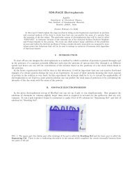
Reweighting: what it is
Do simulations at µ f = 0, re-express expectation values in terms of these—
β
Budapest method
〈O〉 µ
=
〈O exp(−∆S)〉
〈exp(−∆S)〉
where
S = S − ∑ f
Tr log M f ,
Glasgow method
µ
Reweighting done for coarse lattices (N t = 4) and N f = 4, 2 and 2+1.
Chemical potential/S. Gupta: IMSc, 2003 to plan, Phases, Reweight, Expansion, QNS, strangeness, EOS, masses, end 4

Reweighting and other direct approaches
• Two parameter reweighting and results.
Z. Fodor and S. D. Katz, J. H. E. P., 03 (2002) 014.
• Express the reweighting in terms of derivatives of Z with respect to µ.
C. R. Allton et al., Phys. Rev., D 66 (2002) 074507
• Simulate imaginary µ (positive det M) and do analytic continuation.
M. D’Elia and M.-P. Lombardo, hep-lat/0209146
P. De Forcrand and O. Philipsen, Nucl. Phys., B642 (2002) 290
• Special care needed for this: find Yang-Lee zeroes directly.
S, Gupta, hep-lat/0307007.
• Canonical partition functions and propagator matrix.
P. Crompton, P. Higgs, MILC, BI, etc
Chemical potential/S. Gupta: IMSc, 2003 to plan, Phases, Reweight, Expansion, QNS, strangeness, EOS, masses, end 5

Chemical potential/S. Gupta: IMSc, 2003 to plan, Phases, Reweight, Expansion, QNS, strangeness, EOS, masses, end 6

Reweighting: lattice artifacts
Chemical potential on the lattice is prescription dependent. Why? The continuum
Dirac operator specifies effects of an infinitesimal time translation. On the lattice
we deal with finite translations (by lattice spacing a). There are many ways of
doing this which lead to the same infinitesimal transformation.
This is the origin of problems with reweighting: it gives no indication of how large
the lattice artifacts are.
Taylor series expansion is prescription dependent beyond 2nd order at every finite
lattice spacing a, but prescription independent for a → 0. With explicit Taylor
expansion we can take the continuum limit.
R. V. Gavai and S. Gupta, Phys. Rev. D 68 (2003) 034506.
Chemical potential/S. Gupta: IMSc, 2003 to plan, Phases, Reweight, Expansion, QNS, strangeness, EOS, masses, end 7

The Taylor Expansion
Since P V = −F = T log Z, the Taylor expansion of P is the same as of F !
1
V P (T, µ u, µ d ) = 1 V P (T, 0, 0) + ∑ f
n f µ f + 1 2!
where the quark number densities and susceptibilities are—
∑
χ fg µ f µ g + · · ·
fg
n f = T V
χ fg = T V
χ fgh··· = T V
∂ log Z
∂µ f
∣ ∣∣∣µf
=0
∣
∂ 2 log Z ∣∣∣µf
∂µ f ∂µ g =µ g =0
∂ n log Z
∣
∂µ f ∂µ g ∂µ h · · ·
∣
µf =µ g =···=0
Chemical potential/S. Gupta: IMSc, 2003 to plan, Phases, Reweight, Expansion, QNS, strangeness, EOS, masses, end 8

Derivatives
Derivatives of log Z can be expressed in terms of derivatives of Z. The latter can
be constructed by the chain rule.
Z f = ∂Z
∂µ f
=
∫
DUe −S Tr M −1
f M ′ f.
Note: M ′ = γ 0 and M −1 = ψψ, so Tr M −1 M ′ = ψ † ψ. Odd derivatives vanish
for µ f = 0 by CP symmetry. S. Gottlieb et al., Phys. Rev. Lett., 59 (1987) 2247
1 2 11
111 21 3
S. Gupta, Acta Phys. Pol., B 33 (2002) 4259
Chemical potential/S. Gupta: IMSc, 2003 to plan, Phases, Reweight, Expansion, QNS, strangeness, EOS, masses, end 9

Quark number susceptibilities: phenomena
• Fluctuations of conserved quantities in heavy-ion collisions are related to χ uu .
Isospin fluctuations are related to χ 3 = χ uu − χ ud , charge fluctuations can also
be constructed out of these. M. Asakawa et al., Phys. Rev. Lett., 85 (2000) 2072; S.
Jeon and V. Koch, ibid., 85 (2000) 2076
• Under certain conditions strangeness production rate can be related to the
strange susceptibility, χ ss . R. V. Gavai et al., Phys. Rev., D 65 (2002) 054506
• The pressure at finite chemical potential is essentially determined by the
susceptibility. R. V. Gavai and S. Gupta, Phys. Rev. D 68 (2003) 034506.
• χ 3 is the zero momentum Euclidean finite temperature vector propagator and
hence closely related to a transport coefficient— the DC electrical conductivity
of quark matter. S. Gupta, hep-lat/0301006.
Chemical potential/S. Gupta: IMSc, 2003 to plan, Phases, Reweight, Expansion, QNS, strangeness, EOS, masses, end 10

Some notation
With two degenerate flavours of quarks, in flavour space the linear susceptibilities
form the matrix (
χuu χ ud
χ ud χ uu
)
Transforming to µ 0 = µ u + µ d and µ 3 = µ u − µ d , this matrix becomes
(
χuu + χ ud 0
0 χ uu − χ ud
)
χ 3 = χ uu − χ ud = 〈 Tr M −1 M ′ M −1 M ′ − Tr M −1 M ′′〉
χ ud =
〈 (Tr
M −1 M ′) 2 〉 and χ 0 = χ 3 + 2χ ud
Chemical potential/S. Gupta: IMSc, 2003 to plan, Phases, Reweight, Expansion, QNS, strangeness, EOS, masses, end 11

Finding the continuum limit
Main technical problem is to control the extrapolation to zero lattice spacing. For
this we use two different kinds of Fermions (staggered and Naik) and perform
simultaneous extrapolation with both: in the quenched theory.
R. V. Gavai and S. Gupta, Phys. Rev. D 67 (2003) 034501
1.8
1.6
/T 2
χ 3
1.4
1.2
1
0.8
0 0.01 0.02 0.03 0.04 0.05 0.06 0.07
1/N
2
t
Chemical potential/S. Gupta: IMSc, 2003 to plan, Phases, Reweight, Expansion, QNS, strangeness, EOS, masses, end 12

Perturbation theory
1.0
1
0.9
NL
HTL
0.95
χ /Τ 2
3
0.8
0.7
χ uu
/T 2
0.9
0.85
∆ = 2
∆ = 1
∆ = 0
∆ = −1
∆ = −2
Lattice
0.6
1 2 3
T/T c
0.8
1 2 3 4 5
T/T c
J.P. Blaizot, E. Iancu and A. Rebhan, Phys. Lett., B 523 (2001) 143
A. Vuorinen, hep-ph/0212283
Chemical potential/S. Gupta: IMSc, 2003 to plan, Phases, Reweight, Expansion, QNS, strangeness, EOS, masses, end 13

χ ud and χ uu
1.0
1
χ 3 /T 2
0.8
0.6
0.4
0.2
10 5 χ ud /T 2
0.5
0
-0.5
-1
-1.5
0
0.5 1 1.5 2 2.5 3
T/Tc
-2
0.5 1 1.5 2 2.5 3
T/Tc
(Note the difference in scales!)
Chemical potential/S. Gupta: IMSc, 2003 to plan, Phases, Reweight, Expansion, QNS, strangeness, EOS, masses, end 14

Event to event fluctuations
Each heavy-ion collision event, followed by the hadronisation, is one realisation of
the whole ensemble of possible thermodynamic systems. Within a given rapidity
region, the total amount of any conserved charge fluctuates from one event to
another. The variance is determined by the response function of QCD matter in
equilibrium.
M. Asakawa et al., Phys. Rev. Lett., 85 (2000) 2072
S. Jeon et al., Phys. Rev. Lett., 85 (2000) 2076
D. Bower and S. Gavin, Phys. Rev., C 64 (2001) 051902
From lattice computations it is seen that
χ B < χ Q < χ s (T > T c )
χ B > χ Q > χ s (T < T c )
R. V. Gavai, S. Gupta, P. Majumdar, Phys. Rev., D 65 (2002) 054506
Chemical potential/S. Gupta: IMSc, 2003 to plan, Phases, Reweight, Expansion, QNS, strangeness, EOS, masses, end 15

Strangeness production
[ ]
Dynamical QCD (T c )
Quenched QCD (T c )
RHIC Au-Au
SpS S-S
SpS S-Ag
SpS Pb-Pb
AGS Au-Au
AGS Si-Au
0.2 0.4 0.6 0.8 1
λs
J. Cleymans, J. Phys., G 28 (2002) 1575,
λ s = 〈n s〉
〈n u + n d 〉
R. V. Gavai and S. Gupta, Phys. Rev., D 65 (2002) 094515.
Chemical potential/S. Gupta: IMSc, 2003 to plan, Phases, Reweight, Expansion, QNS, strangeness, EOS, masses, end 16

The pressure
P (T, µ) = −F/V = P (T, 0) + χ 3 (T )µ 2 + 1 12 χ uuuu(T )µ 4 + O ( µ 6)
= P (T, 0) +
(
µ
µ (2)
∗
) 2
⎡
⎣1 +
(
µ
µ (4)
∗
) 2
⎧
⎨
⎩ 1 + (
µ
µ (6)
∗
) ⎤
2
⎬
+ · · ·⎫
⎦ .
⎭
where µ (2)
∗ = √ 2/χ uu , µ (4)
∗ = √ 12χ uu /χ uuuu , µ (6)
∗
= √ 30χ uuuu /χ uuuuuu , etc.
Well-behaved for µ ≪ µ ∗ . All results can be obtained in the continuum. Term by
term improvement of the series is possible.
Chemical potential/S. Gupta: IMSc, 2003 to plan, Phases, Reweight, Expansion, QNS, strangeness, EOS, masses, end 17

The equation of state
0.5
100
0.4
1.03
10
1
∆P/T 4
0.3
0.2
0.73
∆ P/T 4
0.1
0.01
1 dP
T dn
0.1
0.44
0.001
0.0001
0
1
0.15
1.5 2 2.5 3
T/T c
0.001 0.01 0.1 1 10
n/T3
∆P (T ) = P (T, µ) − P (T, 0)
R. V. Gavai and S. Gupta, Phys. Rev. D 68 (2003) 034506.
See also
Z. Fodor, S. D. Katz and K. K. Szabo, hep-lat/0208078,
C. R. Allton et al., Phys. Rev., D 68 (2003) 014507.
Chemical potential/S. Gupta: IMSc, 2003 to plan, Phases, Reweight, Expansion, QNS, strangeness, EOS, masses, end 18

Radius of convergence: distance to phase transitions
The series expansion breaks down when a phase transition line is encountered. Use
any estimate of the radius of convergence to obtain an estimate of the position of
the phase transition line.
4
3
/T
*
µ n
2
1
0.95Tc
2Tc
0
0 2 4 6 8 10
n
Qualitative difference between T < T c and T > T c ?
Chemical potential/S. Gupta: IMSc, 2003 to plan, Phases, Reweight, Expansion, QNS, strangeness, EOS, masses, end 19

Condensates and masses
Taylor expansions can also be made for expectation values of any operator. We
are investigating this for
1. Condensates: 〈ψψ〉 changes quadratically with µ, and the quadratic coefficient
is the same for isovector and baryon chemical potential. This number is also
related to λ s in strangeness production through a Maxwell relation.
2. Masses: The mass splitting of charged pions at finite isovector chemical
potential is linear in µ, but that of the neutral pion is quadratic. This quadratic
coefficient is the same as shift in pion mass at finite baryon chemical potential.
O. Miyamura et al., Phys. Rev., D 66 (2002) 077502,
S. Gupta, hep-lat/0202005, S. Gupta and Rajarshi Ray, in progress
Chemical potential/S. Gupta: IMSc, 2003 to plan, Phases, Reweight, Expansion, QNS, strangeness, EOS, masses, end 20

Summary of Results
More than one method for computing physics at finite µ. One method (Taylor
series expansion) is a precision technique, allowing contact with experiments.
• Computation of several high order susceptibilities may allow estimation of the
critical end point by series extrapolation methods.
• Fluctuations and strangeness production rate in heavy-ion collisions are related
to susceptibilities.
• Susceptibilities allow extension of the equation of state to finite chemical
potential.
• Taylor expansions yield identities between behaviour of various quantities at
finite isovector and baryon chemical potential.
Chemical potential/S. Gupta: IMSc, 2003 to plan, Phases, Reweight, Expansion, QNS, strangeness, EOS, masses, end 21