1309 KB pdf file - Department of Theoretical Physics - Tata Institute ...
1309 KB pdf file - Department of Theoretical Physics - Tata Institute ...
1309 KB pdf file - Department of Theoretical Physics - Tata Institute ...

You also want an ePaper? Increase the reach of your titles
YUMPU automatically turns print PDFs into web optimized ePapers that Google loves.
Non Supersymmetric Attractors<br />
A thesis submitted to the<br />
<strong>Tata</strong> <strong>Institute</strong> <strong>of</strong> Fundamental Research, Mumbai<br />
for the degree <strong>of</strong><br />
PhD, in <strong>Physics</strong><br />
by<br />
Rudra Pratap Jena<br />
<strong>Department</strong> <strong>of</strong> <strong>Theoretical</strong> <strong>Physics</strong>, School <strong>of</strong> Natural Sciences<br />
<strong>Tata</strong> <strong>Institute</strong> <strong>of</strong> Fundamental Research, Mumbai<br />
Aug, 2007
I dedicate this thesis to my parents.
Acknowledgements<br />
It is a pleasure to thank the many people who made this thesis possible.<br />
It is difficult to overstate my gratitude to my Ph.D. supervisor, Sandip<br />
Trivedi. With his enthusiasm, his inspiration, and his great efforts to<br />
explain things clearly and simply, he helped to make physics fun for<br />
me. Throughout my PhD period, he provided encouragement, sound<br />
advice, good teaching, good company, and lots <strong>of</strong> good ideas. I would<br />
have been lost without him. I could not have imagined having a<br />
better advisor and mentor for my PhD, and without his knowledge,<br />
perceptiveness and cracking-<strong>of</strong>-the-whip I would never have finished.<br />
I would like to mention special thanks to Norihiro Iizuka, Kevin Goldstein,<br />
Ashoke Sen and Gautam Mandal who have taught me lot <strong>of</strong><br />
physics, during my work with them.<br />
I thank all my teachers for inspiring me to do physics. I have really<br />
benefitted from various stimulating discussions in TIFR string theory<br />
group. It was exciting to attend all those string lunches and string<br />
theory seminars. I have learnt a lot <strong>of</strong> physics during these, thanks to<br />
Sunil Mukhi, Shiraz Minwalla, Atish Dabholkar, Spenta Wadia and<br />
Avinash Dhar.<br />
I am indebted to my many student colleagues for providing a stimulating<br />
and fun environment in which to learn and grow. I am especially<br />
grateful to Pallab Basu, Basudeb Dasgupta, Aniket Basu,<br />
Rahul Nigam, Anindya Mukherji, Shamik Gupta, Sashideep Gutti,<br />
Suresh Nampuri, Loganayagam, Sayantani, Partha, Debasish, Jyotirmoy<br />
from TIFR, Suvrat Raju, Lars Grant, Subhaniel Lahiri, Joe
Marsano and Kyriakos from Harvard, Liam Mcallister from Stanford<br />
and Matthew Buican from Princeton. I would also like to thank my<br />
batchmates at TIFR, who made my stay really memorable, Sourin,<br />
Ravi, Subhendu and Kelkar.<br />
I am grateful to the secretaries in the <strong>Department</strong> <strong>of</strong> <strong>Theoretical</strong><br />
<strong>Physics</strong>, for helping the department to run smoothly and for assisting<br />
me in many different ways. Raju Bathija, Girish Ogale, Pawar and<br />
Shinde, all deserve special mention.<br />
I wish to thank my entire extended family for providing a loving environment<br />
for me. My sister and some first cousins were particularly<br />
supportive. I also wish to thank Farheen for her invaluable support<br />
at times.<br />
Lastly, and most importantly, I wish to thank my parents. They raised<br />
me, supported me, taught me, and loved me. To them I dedicate this<br />
thesis.
Contents<br />
1 Introduction 1<br />
1.1 Outline <strong>of</strong> the Thesis . . . . . . . . . . . . . . . . . . . . . . . . . 4<br />
2 Non Supersymmetric Attractors 12<br />
2.1 Attractor in Four-Dimensional Asymptotically Flat Space . . . . . 12<br />
2.1.1 Equations <strong>of</strong> Motion . . . . . . . . . . . . . . . . . . . . . 12<br />
2.1.2 Conditions for an Attractor . . . . . . . . . . . . . . . . . 16<br />
2.1.3 Comparison with the N = 2 Case . . . . . . . . . . . . . . 18<br />
2.1.4 Perturbative Analysis . . . . . . . . . . . . . . . . . . . . . 19<br />
2.1.4.1 A Summary . . . . . . . . . . . . . . . . . . . . . 19<br />
2.1.4.2 First Order Solution . . . . . . . . . . . . . . . . 21<br />
2.1.4.3 Second Order Solution . . . . . . . . . . . . . . . 22<br />
2.1.4.4 An Ansatz to All Orders . . . . . . . . . . . . . . 24<br />
2.2 Numerical Results . . . . . . . . . . . . . . . . . . . . . . . . . . . 27<br />
2.3 Exact Solutions . . . . . . . . . . . . . . . . . . . . . . . . . . . . 30<br />
2.3.1 Explicit Form <strong>of</strong> the f i . . . . . . . . . . . . . . . . . . . . 33<br />
2.3.2 Supersymmetry and the Exact Solutions . . . . . . . . . . 33<br />
2.4 General Higher Dimensional Analysis . . . . . . . . . . . . . . . . 34<br />
2.4.1 The Set-Up . . . . . . . . . . . . . . . . . . . . . . . . . . 34<br />
2.4.2 Zeroth and First Order Analysis . . . . . . . . . . . . . . . 35<br />
2.4.2.1 Second order calculations (Effects <strong>of</strong> backreaction) 36<br />
2.5 Attractor in AdS 4 . . . . . . . . . . . . . . . . . . . . . . . . . . . 38<br />
2.5.1 Zeroth and First Order Analysis for V . . . . . . . . . . . 39<br />
2.6 Additional Comments . . . . . . . . . . . . . . . . . . . . . . . . 42<br />
2.7 Asymptotic de Sitter Space . . . . . . . . . . . . . . . . . . . . . 44<br />
iv
CONTENTS<br />
2.7.1 Perturbation Theory . . . . . . . . . . . . . . . . . . . . . 45<br />
2.7.2 Some Speculative Remarks . . . . . . . . . . . . . . . . . . 46<br />
2.8 Non-Extremal = Unattractive . . . . . . . . . . . . . . . . . . . . 47<br />
2.9 Perturbation Analysis . . . . . . . . . . . . . . . . . . . . . . . . 51<br />
2.9.1 Mass . . . . . . . . . . . . . . . . . . . . . . . . . . . . . . 51<br />
2.9.2 Perturbation Series to All Orders . . . . . . . . . . . . . . 52<br />
2.10 Exact Analysis . . . . . . . . . . . . . . . . . . . . . . . . . . . . 53<br />
2.10.1 New Variables . . . . . . . . . . . . . . . . . . . . . . . . . 53<br />
2.10.2 Equivalent Toda System . . . . . . . . . . . . . . . . . . . 54<br />
2.10.3 Solutions . . . . . . . . . . . . . . . . . . . . . . . . . . . . 55<br />
2.10.3.1 Case I: γ = 1 ⇔ α 1 α 2 = −4 . . . . . . . . . . . . 55<br />
2.10.3.2 Case II: γ = 2 and α 1 = −α 2 = 2 √ 3 . . . . . . . 56<br />
2.10.3.3 Case III: γ = 3 and α 1 = 4 α 2 = −6 . . . . . 58<br />
2.11 Higher Dimensions . . . . . . . . . . . . . . . . . . . . . . . . . . 60<br />
2.12 More Details on Asymptotic AdS Space . . . . . . . . . . . . . . . 62<br />
3 C- function for Non-Supersymmetric Attractors 64<br />
3.1 Background . . . . . . . . . . . . . . . . . . . . . . . . . . . . . . 64<br />
3.2 The c-function in 4 Dimensions. . . . . . . . . . . . . . . . . . . 67<br />
3.2.1 The c-function . . . . . . . . . . . . . . . . . . . . . . . . 67<br />
3.2.2 Some Comments . . . . . . . . . . . . . . . . . . . . . . . 68<br />
3.3 The c-function In Higher Dimensions . . . . . . . . . . . . . . . . 72<br />
3.4 Concluding Comments . . . . . . . . . . . . . . . . . . . . . . . . 76<br />
3.5 V eff Need Not Be Monotonic . . . . . . . . . . . . . . . . . . . . 79<br />
3.6 More Details in Higher Dimensional Case . . . . . . . . . . . . . . 82<br />
3.7 Higher Dimensional p-Brane Solutions . . . . . . . . . . . . . . . 83<br />
4 Rotating Attractors 85<br />
4.1 General Analysis . . . . . . . . . . . . . . . . . . . . . . . . . . . 85<br />
4.2 Extremal Rotating Black Hole in General Two Derivative Theory 93<br />
4.3 Solutions with Constant Scalars . . . . . . . . . . . . . . . . . . . 100<br />
4.3.1 Extremal Kerr Black Hole in Einstein Gravity . . . . . . . 104<br />
4.3.2 Extremal Kerr-Newman Black Hole in Einstein-Maxwell<br />
Theory . . . . . . . . . . . . . . . . . . . . . . . . . . . . . 105<br />
v
CONTENTS<br />
4.4 Examples <strong>of</strong> Attractor Behaviour in Full Black Hole Solutions . . 105<br />
4.4.1 Rotating Kaluza-Klein Black Holes . . . . . . . . . . . . . 106<br />
4.4.1.1 The black hole solution . . . . . . . . . . . . . . 107<br />
4.4.1.2 Extremal limit: The ergo-free branch . . . . . . . 109<br />
4.4.1.3 Near horizon behaviour . . . . . . . . . . . . . . 110<br />
4.4.1.4 Entropy function analysis . . . . . . . . . . . . . 112<br />
4.4.1.5 The ergo-branch . . . . . . . . . . . . . . . . . . 113<br />
4.4.2 Black Holes in Toroidally Compactified Heterotic String<br />
Theory . . . . . . . . . . . . . . . . . . . . . . . . . . . . . 118<br />
4.4.2.1 The black hole solution . . . . . . . . . . . . . . 120<br />
4.4.2.2 The ergo-branch . . . . . . . . . . . . . . . . . . 122<br />
4.4.2.3 The ergo-free branch . . . . . . . . . . . . . . . . 123<br />
4.4.2.4 Duality invariant form <strong>of</strong> the entropy . . . . . . . 124<br />
5 Extension to black rings 126<br />
5.1 Black thing entropy function and dimensional reduction . . . . . . 126<br />
5.2 Algebraic entropy function analysis . . . . . . . . . . . . . . . . . 128<br />
5.2.1 Set up . . . . . . . . . . . . . . . . . . . . . . . . . . . . . 129<br />
5.2.2 Preliminary analysis . . . . . . . . . . . . . . . . . . . . . 131<br />
5.2.3 Black rings . . . . . . . . . . . . . . . . . . . . . . . . . . 132<br />
5.2.3.1 Magnetic potential . . . . . . . . . . . . . . . . . 134<br />
5.2.4 Static 5-d black holes . . . . . . . . . . . . . . . . . . . . . 135<br />
5.2.4.1 Electric potential . . . . . . . . . . . . . . . . . . 137<br />
5.2.5 Very Special Geometry . . . . . . . . . . . . . . . . . . . . 137<br />
5.2.5.1 Black rings and very special geometry . . . . . . 137<br />
5.2.5.2 Static black holes and very special geometry . . . 138<br />
5.2.5.3 Non-supersymmetric solutions <strong>of</strong> very special geometry<br />
. . . . . . . . . . . . . . . . . . . . . . . . 139<br />
5.2.5.4 Rotating black holes . . . . . . . . . . . . . . . . 140<br />
5.3 General Entropy function . . . . . . . . . . . . . . . . . . . . . . 141<br />
5.4 Supersymmetric black ring near horizon geometry . . . . . . . . . 141<br />
5.5 Notes on Very Special Geometry . . . . . . . . . . . . . . . . . . . 145<br />
5.6 Spinning black hole near horizon geometry . . . . . . . . . . . . . 147<br />
vi
CONTENTS<br />
5.7 Non-supersymmetric ring near horizon geometry . . . . . . . . . . 148<br />
5.7.1 Near horizon geometry . . . . . . . . . . . . . . . . . . . . 150<br />
6 Conclusions 153<br />
References 161<br />
vii
Chapter 1<br />
Introduction<br />
Black holes provide an interesting area to explore the challenges which arise in<br />
attempts to reconcile general relativity and quantum mechanics. Since string theory<br />
includes within its framework a quantum theory <strong>of</strong> gravity, it should be able<br />
to address these challenges. In fact, some <strong>of</strong> the most fascinating developments<br />
in string theory concerns black hole physics. Classically, black holes are solutions<br />
to Einstein’s equations <strong>of</strong> general relativity, which have an event horizon. Due to<br />
the intense gravitational pull <strong>of</strong> the black hole, nothing can escape from inside<br />
this horizon.<br />
Let us begin with the simplest black hole solutions <strong>of</strong> Einstein’s equations in four<br />
dimensions, which are the Schwarzschild and Reissner-Nordstrom black holes.<br />
In four dimensions the Schwarzschild black hole metric, in Schwarzschild coordinates<br />
is,<br />
ds 2 = −(1 − r H<br />
r )dt2 + (1 − r H<br />
r )−1 dr 2 + r 2 dΩ 2 2. (1.1)<br />
where r H = 2G 4 M.<br />
Here r H is known as Schwarzschild radius and G 4 is Newton’s constant and M<br />
is the mass <strong>of</strong> the black hole. Here t is a timelike coordinate for r > r H and<br />
spacelike for r < r H , while reverse is true for r. The surface r = r H is called the<br />
event horizon, which seperates these two regions.<br />
The generalisation <strong>of</strong> the Schwarzschild black hole to one with electric charge Q,<br />
is called the Reissner-Nordstrom black hole. In four dimensions, the metric <strong>of</strong><br />
1
Reissner-Nordstrom black hole takes the form,<br />
where ∆ = 1 − 2M + Q2<br />
.<br />
r r 2<br />
The g tt component <strong>of</strong> the metric vanishes for,<br />
s 2 = −∆dt 2 + ∆ −1 dr 2 + r 2 dΩ 2 2, (1.2)<br />
r = r ± = M ± √ M 2 − Q 2 (1.3)<br />
which are the inner and outer horizons respectively. The outer horizon r = r + is<br />
the event horizon. It is only present if<br />
M ≥ |Q| (1.4)<br />
In the limiting case<br />
r ± = M or M = |Q| (1.5)<br />
the black hole is called extremal, and it has minimum mass allowed given its<br />
charge, as follows from the bound (1.4). For a general charge configuration, an<br />
extremal black hole configuration is one with lowest mass allowed by the charges.<br />
The metric <strong>of</strong> the extremal Reissner-Nordstrom black hole takes the form,<br />
ds 2 = −(1 − r 0<br />
r )2 dt 2 + (1 − r 0<br />
r )−2 dr 2 + r 2 dΩ 2 2 . (1.6)<br />
where r 0 = M. In the near horizon limit, where r ≈ 0, the geometry approaches<br />
AdS 2 × S 2 .<br />
The mass M and charge Q <strong>of</strong> the black hole are defined in terms <strong>of</strong> appropriate<br />
surface integrals at spatial infinity. Two important quantities associated with the<br />
black hole horizon are its area A and the surface gravity κ s . The surface gravity,<br />
which is constant on the horizon, is related to the force(measured at spatial infinity)<br />
that holds a unit test mass in place.<br />
Classical black holes behave like thermodynamic systems characterised by temperature<br />
and entropy. Let us first consider the thermodynamic description, i.e.,<br />
the macroscopic description <strong>of</strong> black holes.<br />
The first law for thermodynamics<br />
states that the variation <strong>of</strong> the total energy is equal to the temperature times the<br />
variation <strong>of</strong> the entropy plus work terms. The corresponding formula for black<br />
holes states that the variation <strong>of</strong> black hole mass is related to the variation <strong>of</strong><br />
2
the horizon area plus the work terms proportional to the variation <strong>of</strong> the angular<br />
momentum and a term proportional to a variation <strong>of</strong> the charge, multiplied by<br />
the electric/magnetic potential µ at the horizon.<br />
δM = κ s δA<br />
+ µδQ + ΩδJ. (1.7)<br />
2π 4<br />
It was found by Hawking [1] that any black hole emits radiation with the spectrum<br />
<strong>of</strong> a black body at temperature κ s /2π. This leads to the identification <strong>of</strong> the black<br />
hole entropy in terms <strong>of</strong> the horizon area,<br />
S macro = 1 4 A (1.8)<br />
This relation, known as Bekenstein-Hawking entropy, appears to be universally<br />
valid, atleast when A is sufficiently large.<br />
This identification raises the question what the black hole microstates are,<br />
and where they are located. We want to know what the statistical mechanics<br />
<strong>of</strong> black holes is, and express (1.8) as the logarithm <strong>of</strong> a number <strong>of</strong> microstates<br />
that are compatible with a given macrostate, i.e., a black hole with a given set<br />
(M, J, Q). String theory provides a microscopic quantum description <strong>of</strong> some supersymmetric<br />
black holes. For these black holes, the logarithm <strong>of</strong> the degeneracy<br />
<strong>of</strong> states as a function <strong>of</strong> charge Q, d(Q), has been shown to exactly match the<br />
Bekenstein-Hawking entropy in the limit <strong>of</strong> large charges. The first microstate<br />
counting for black holes in string theory that reproduced the right numerical<br />
coefficent <strong>of</strong> the Bekenstein Hawking entropy was done by Strominger and Vafa<br />
. They considered supersymmetric (and thus necessarily extremal and charged)<br />
black holes. In the presence <strong>of</strong> supersymmetry, there exists non renormalization<br />
theorems, which essentially say that the weak coupling results are protected<br />
from quantum corrections. This means that the number <strong>of</strong> states one counts at<br />
weak coupling cannot change as one increases the coupling, i.e., when a black<br />
hole forms. These microstates correspond to configuration <strong>of</strong> wrapped branes.<br />
More recently, it has been shown that the Bekenstein Hawking Wald entropy for<br />
a number <strong>of</strong> black hole examples, agree to all orders in preturbation theory in<br />
inverse charges going well beyond the perturbation limit.<br />
3
1.1 Outline <strong>of</strong> the Thesis<br />
Supersymmetric black holes are well known to exhibit a striking phenomenon<br />
called the attractor behavior [2, 3, 4]. Moduli fields in these black hole backgrounds<br />
take value at the horizon independent <strong>of</strong> their asymptotic values at infinity,<br />
determined by the charges only. As a result, the macroscopic entropy<br />
depends only on the charges. This is consistent with the fact that the microscopic<br />
entropy, more precisely, an index is also independent <strong>of</strong> the asymptotic<br />
moduli due to the BPS property <strong>of</strong> the states.<br />
So far the attractor mechanism has been studied almost exclusively in the context<br />
<strong>of</strong> N = 2 supergravity. The question which interests us in this thesis is if this<br />
mechanism is more general. We want to study whether it works for non supersymmetric<br />
black holes as well. The extremal black holes have some properties<br />
which are similar to supersymmetric black holes, for example they have vanishing<br />
surface gravity and have the minimal possible mass compatible with the given<br />
charges and angular momentum. This motivates the search <strong>of</strong> attractor behavior<br />
in extremal configurations. We investigate the attractor mechanism for extremal<br />
black holes and black rings in two derivative actions describing gravity coupled<br />
to scalar fields and abelian gauge fields. These black holes might be solutions in<br />
theories which have no supersymmetry or might be non supersymmetric solutions<br />
in supersymmetric theories.<br />
1.1 Outline <strong>of</strong> the Thesis<br />
The theories we consider consist <strong>of</strong> gravity, gauge fields and scalar fields with the<br />
action<br />
S = 1 κ 2 ∫<br />
d 4 x √ −G(R−2(∂φ i ) 2 −f ab (φ i )F a µνF b µν − 1 2 ˜f ab (φ i )F a µνF b ρσɛ µνρσ ). (1.9)<br />
Here the index i denotes the different scalars and a, b the different gauge fields<br />
and Fµν a stands for the field strength <strong>of</strong> the gauge field. f ab(φ i ) determines the<br />
gauge couplings and ˜f ab (φ i ) determines the axionic couplings.<br />
The scalars determine the gauge couplings and thereby couple to the gauge fields.<br />
4
1.1 Outline <strong>of</strong> the Thesis<br />
It is important that the scalars do not have a potential <strong>of</strong> their own that gives<br />
them in particular a mass. Such a potential would mean that the scalars are no<br />
longer moduli.<br />
The theories described by (1.9), are four dimensional and do not have a cosmological<br />
constant. This action can be generalized to higher dimensions as well<br />
as theories with cosmological constant. In chapter 2, we explore the attractor<br />
mechanism in spherical symmetric extremal black holes for theories mentioned<br />
in (1.9) [5]. The moduli fields in a black hole background vary radially and get<br />
attracted to specific values at the horizon, which depends only on the charges.<br />
The attractor behavior also refers to the fact that the near horizon geometry<br />
approaches AdS 2 × S 2 and the AdS 2 and S 2 radii depend only on the charges.<br />
We show that the attractor mechanism works quite generally in such theories<br />
provided two conditions are met. These conditions are succinctly stated in terms<br />
<strong>of</strong> an “effective potential” V eff for the scalar fields, φ i .<br />
With both electric and magnetic charges the gauge fields take the form,<br />
F a = f ab (φ i )(Q eb − ˜f bc Q c m) 1 b dt ∧ dr + 2 Qa msinθdθ ∧ dφ, (1.10)<br />
where Q a m, Q ea are constants that determine the magnetic and electric charges<br />
carried by the gauge field F a , and f ab is the inverse <strong>of</strong> f ab .<br />
The effective potential is then given by,<br />
V eff (φ i ) = f ab (Q ea − ˜f ac Q c m)(Q eb − ˜f bd Q d m) + f ab Q a mQ b m. (1.11)<br />
The effective potential is proportional to the energy density in the electromagnetic<br />
field and arises after solving for the gauge fields in terms <strong>of</strong> the charges<br />
carried by the black hole. The two conditions that need to be met are the following.<br />
First, as a function <strong>of</strong> the moduli fields V eff must have a critical point,<br />
∂ i V eff (φ i0 ) = 0. And second, the matrix <strong>of</strong> second derivatives <strong>of</strong> the effective potential<br />
at the critical point, ∂ ij V eff (φ i0 ), must be have only positive eigenvalues.<br />
The resulting attractor values for the moduli are the critical values, φ i0 . And the<br />
entropy <strong>of</strong> the black hole is proportional to V (φ i0 ), and is thus independent <strong>of</strong><br />
the asymptotic values for the moduli. It is worth noting that the two conditions<br />
stated above are met by BPS black hole attractors in an N = 2 supersymmetric<br />
theory.<br />
5
1.1 Outline <strong>of</strong> the Thesis<br />
The analysis for BPS attractors simplifies greatly due to the use <strong>of</strong> the first<br />
order equations <strong>of</strong> motion. In the non-supersymmetric context one has to work<br />
with the second order equations directly and this complicates the analysis. The<br />
central idea in establishing the attractor behavior lies in the perturbation analysis.<br />
Although the equations are second order, in perturbation theory they are linear,<br />
and this makes them tractable. For the static spherically symmetric case, we can<br />
consistently set the scalars to their critical values for all values <strong>of</strong> r. This gives<br />
rise to an extremal Reissner Nordstrom black hole. If the scalar field takes value<br />
at asymptotic infinity which are small deviations from their attractor values, we<br />
show that the extremal black hole solution continues to exist. The scalar takes<br />
the attractor value at the horizon. The analysis can be carried out quite generally<br />
for any effective potential for the scalars and shows that the two conditions stated<br />
above are sufficient for the attractor phenomenon to hold.<br />
We also carry out numerical analysis to go beyond the perturbation results.<br />
This requires a specific form <strong>of</strong> the effective potential. The numerical analysis<br />
corroborates the perturbation theory results mentioned above. In simple cases we<br />
have explored so far, we have found evidence for a only single basin <strong>of</strong> attraction,<br />
although multiple basins must exist in general as is already known from the<br />
supersymmetric(SUSY) cases.<br />
We generalize these results to other settings. We find that the attractor<br />
phenomenon continues to hold in higher dimensions and Anti-de Sitter space<br />
(AdS), as long as the two conditions mentioned above are valid for a suitable<br />
defined effective potential.<br />
For a completely general class <strong>of</strong> gravity actions including higher derivative<br />
interactions, assuming an extremal near horizon geometry <strong>of</strong> form AdS 2 × S 2<br />
but without assuming supersymmetry, the attractor values <strong>of</strong> the moduli can be<br />
obtained by extremizing an “entropy function”[6]. For the two derivative theories,<br />
the entropy function and the effective potential are different quantities, but the<br />
extremisation results give the same attractor values.<br />
In chapter 2, we construct an effective potential for extremal black holes, which<br />
is minimized with respect to the moduli to get the attractor values <strong>of</strong> the scalars.<br />
For supersymmetric black holes, there is a function <strong>of</strong> the moduli and the charges<br />
carried by the black hole, called the central charge, which plays an important<br />
6
1.1 Outline <strong>of</strong> the Thesis<br />
Figure 1.1: Variation <strong>of</strong> the scalar moduli as we move in from infinity into the<br />
horizon.<br />
role in the discussion <strong>of</strong> the attractor. The attractor values <strong>of</strong> the scalars, which<br />
are obtained at the horizon <strong>of</strong> the black hole, are given by minimizing the central<br />
charge with respect to the moduli.<br />
There is a another sense in which the central charge is also minimized at the<br />
horizon <strong>of</strong> a supersymmetric attractor. One finds that the central charge, now<br />
regarded as a function <strong>of</strong> the position coordinate, evolves monotonically from<br />
asymptotic infinity to the horizon and obtains its minimum value at the horizon<br />
<strong>of</strong> the black hole. It is natural to ask whether there is an analogous quantity in<br />
the non-supersymmetric case and in particular if the effective potential is also<br />
monotonic and minimized in this sense for non-supersymmetric attractors.<br />
In chapter 3, we propose a c-function for non-supersymmetric spherically symmetric<br />
attractors. We first study the four dimensional case. The c-function has a<br />
simple geometrical and physical interpretation in this case. We are interested in<br />
spherically symmetric and static configurations in which all fields are functions<br />
<strong>of</strong> only one variable - the radial coordinate. The c-function, c(r), is given by<br />
7
1.1 Outline <strong>of</strong> the Thesis<br />
c(r) = 1 A(r), (1.12)<br />
4<br />
where A(r) is the area <strong>of</strong> the two-sphere, <strong>of</strong> the SO(3) isometry group orbit,<br />
as a function <strong>of</strong> the radial coordinate 1 . For any asymptotically flat solution we<br />
show that the area function satisfies a c-theorem and monotonically decreases<br />
as one moves towards the horizon, which is the direction <strong>of</strong> increasing redshift<br />
from infinity. For a black hole solution, the static region ends at the horizon,<br />
so in the static region the c-function attains its minimum value at the horizon.<br />
This horizon value <strong>of</strong> the c-function equals the entropy <strong>of</strong> the black hole. While<br />
the horizon value <strong>of</strong> the c-function is also proportional to the minimum value<br />
<strong>of</strong> the effective potential, more generally, away from the horizon, the two are<br />
different. In fact we find that the effective potential need not vary monotonically<br />
in a non-supersymmetric attractor. The c-theorem we prove is applicable<br />
for supersymmetric black holes as well. In the supersymmetric case, there are<br />
three quantities <strong>of</strong> interest, the c-function, the effective potential and the square<br />
<strong>of</strong> the central charge.<br />
At the horizon these are all equal, up to a constant <strong>of</strong><br />
proportionality. But away from the horizon they are in general different.<br />
We work directly with the second order equations <strong>of</strong> motion in our analysis<br />
and it might seem puzzling at first that one can prove a c-theorem at all. The<br />
answer to the puzzle lies in boundary conditions. For black hole solutions we<br />
require that the solutions are asymptotically flat. This is enough to ensure that<br />
going inwards to the horizon from asymptotic infinity the c-function decreases<br />
monotonically.<br />
We generalize the c-function to higher dimensions. We analyze a system <strong>of</strong><br />
rank q gauge fields and moduli coupled to gravity and once again find a c-function<br />
that satisfies a c-theorem. In D = p + q + 1 dimensions this system has extremal<br />
black brane solutions whose near horizon geometry is AdS p+1 ×S q . We show that<br />
the c-function is non-increasing from infinity up to the near horizon region. It’s<br />
minimum value in the AdS p+1 × S q region agrees with the conformal anomaly in<br />
the dual boundary theory for p even [7].<br />
1 We have set G N = 1.<br />
8
1.1 Outline <strong>of</strong> the Thesis<br />
In the first two chapters, we analyse the spherically symmetric configurations.<br />
In chapter 4 we extend the study <strong>of</strong> the attractor mechanism to rotating black hole<br />
solutions. Our starting point is an observation made in [8] that the near horizon<br />
geometries <strong>of</strong> extremal Kerr and Kerr-Newman black holes have SO(2,1)×U(1)<br />
isometry. Armed with this observation we prove a general result that is as powerful<br />
as its non-rotating counterpart. In the context <strong>of</strong> 3+1 dimensional theories,<br />
our analysis shows that in an arbitrary theory <strong>of</strong> gravity coupled to abelian gauge<br />
fields and neutral scalar fields with a gauge and general coordinate invariant local<br />
Lagrangian density, the entropy <strong>of</strong> a rotating extremal black hole remains invariant,<br />
except for occasional jumps, under continuous deformation <strong>of</strong> the asymptotic<br />
data for the moduli fields if an extremal black hole is defined to be the one whose<br />
near horizon field configuration has SO(2, 1) × U(1) isometry.<br />
The strategy for obtaining this result is to use the entropy function formalism<br />
[6]. We find that the near horizon background <strong>of</strong> a rotating extremal black hole<br />
is obtained by extremizing a functional <strong>of</strong> the background fields on the horizon,<br />
and that Bekenstein Hawking entropy is given by precisely the same functional<br />
evaluated at its extremum. Thus if this functional has a unique extremum with<br />
no flat directions then the near horizon field configuration is determined completely<br />
in terms <strong>of</strong> the charges and angular momentum, with no possibility <strong>of</strong><br />
any dependence on the asymptotic data on the moduli fields. On the other hand<br />
if the functional has flat directions so that the extremization equations do not<br />
determine the near horizon background completely, then there can be some dependence<br />
<strong>of</strong> this background on the asymptotic data, but the entropy, being equal<br />
to the value <strong>of</strong> the functional at the extremum, is still independent <strong>of</strong> this data.<br />
Finally, if the functional has several extrema at which it takes different values,<br />
then for different ranges <strong>of</strong> asymptotic values <strong>of</strong> the moduli fields the near horizon<br />
geometry could correspond to different extrema. In this case as we move<br />
in the space <strong>of</strong> asymptotic data the entropy would change discontinuously as we<br />
cross the boundary between two different domains <strong>of</strong> attraction, although within<br />
a given domain it stays fixed. The stability analysis <strong>of</strong> the rotating attractors<br />
has not been done.<br />
We explore this formalism in detail in the context <strong>of</strong> an arbitrary two derivative<br />
theory <strong>of</strong> gravity coupled to scalar and abelian vector fields. The extrem-<br />
9
1.1 Outline <strong>of</strong> the Thesis<br />
ization conditions now reduce to a set <strong>of</strong> second order differential equations with<br />
parameters and boundary conditions which depend only on the charges and the<br />
angular momentum. Thus the only ambiguity in the solution to these differential<br />
equations arise from undetermined integration constants. We prove explicitly that<br />
in a generic situation all the integration constants are fixed once we impose the<br />
appropriate boundary conditions and smoothness requirement on the solutions.<br />
We also show that even in a non-generic situation where some <strong>of</strong> the integration<br />
constants are not fixed (and hence could depend on the asymptotic data on the<br />
moduli fields), the value <strong>of</strong> the entropy is independent <strong>of</strong> these undetermined<br />
integration constants.<br />
We test our general results for some known examples. Here we take some<br />
<strong>of</strong> the known extremal rotating black hole solutions in two derivative theories <strong>of</strong><br />
gravity coupled to matter, and study their near horizon geometry to determine if<br />
they exhibit attractor behavior. We focus on two particular classes <strong>of</strong> examples<br />
— the Kaluza-Klein black holes studied in [9, 10] and black holes in toroidally<br />
compactified heterotic string theory studied in [11]. In both these examples,<br />
we find two kinds <strong>of</strong> extremal limits. One <strong>of</strong> these branches does not have an<br />
ergo-sphere . We call this the ergo-free branch. The other branch does have an<br />
ergo-sphere. We call this the ergo-branch. On both branches the entropy turns<br />
out to be independent <strong>of</strong> the asymptotic values <strong>of</strong> the moduli fields, in accordance<br />
with our general arguments. We find however that while on the ergo-free branch<br />
the scalar and all other background fields at the horizon are independent <strong>of</strong> the<br />
asymptotic data on the moduli fields, this is not the case for the ergo-branch.<br />
Thus on the ergo-free branch we have the full attractor behavior, whereas on<br />
the ergo-branch only the entropy is attracted to a fixed value independent <strong>of</strong> the<br />
asymptotic data.<br />
In five dimensions, one has a black hole with an event horizon <strong>of</strong> topology<br />
S 1 × S 2 , which is called a black ring. Ref[12] obtained an explicit solution <strong>of</strong> five<br />
dimensional vacuum general relativity describing such an object.<br />
By examining the BPS equations for black rings, [13], found the attractor<br />
equations for supersymmetric extremal black rings. Motivated by the results <strong>of</strong><br />
our analysis for black holes, which demonstrate the attractor mechanism is independent<br />
<strong>of</strong> supersymmetry, we extend our analysis to extremal black rings [14]<br />
10
1.1 Outline <strong>of</strong> the Thesis<br />
in chapter 5.<br />
We start with five dimensional Lagrangian consisting <strong>of</strong> gravity, abelian gauge<br />
fields, neutral massless scalars and a Chern-Simons term. We dimensionally reduce<br />
it to four dimensions. Then we apply the entropy function formalism. We<br />
study extremal black rings whose near horizon geometry have AdS 2 × S 2 × U(1)<br />
symmetries. After dimensional reduction, we get an AdS 2 × S 2 near horizon geometry.<br />
This analysis is extended to the five dimensional extremal rotating black<br />
holes. In all these cases, we demonstrate the attractor mechanism for black rings<br />
with out recourse to supersymmetry by using the entropy function formalism.<br />
11
Chapter 2<br />
Non Supersymmetric Attractors<br />
In this chapter, we consider theories with gravity, gauge fields and scalars in fourdimensional<br />
asymptotically flat space-time. By studying the equations <strong>of</strong> motion<br />
directly we show that the attractor mechanism can work for non-supersymmetric<br />
extremal black holes. Two conditions are sufficient for this, they are conveniently<br />
stated in terms <strong>of</strong> an effective potential involving the scalars and the charges<br />
carried by the black hole. Our analysis applies to black holes in theories with<br />
N 1 supersymmetry, as well as non-supersymmetric black holes in theories with<br />
N = 2 supersymmetry. Similar results are also obtained for extremal black holes<br />
in asymptotically Anti-de Sitter space and in higher dimensions.<br />
2.1 Attractor in Four-Dimensional Asymptotically<br />
Flat Space<br />
2.1.1 Equations <strong>of</strong> Motion<br />
In this section we consider gravity in four dimensions with U(1) gauge fields and<br />
scalars. The scalars are coupled to gauge fields with dilaton-like couplings. It<br />
is important for the discussion below that the scalars do not have a potential so<br />
that there is a moduli space obtained by varying their values.<br />
The action we start with has the form,<br />
S = 1 κ 2 ∫<br />
d 4 x √ −G(R − 2(∂φ i ) 2 − f ab (φ i )F a µν F b µν ) (2.1)<br />
12
2.1 Attractor in Four-Dimensional Asymptotically Flat Space<br />
Here the index i denotes the different scalars and a, b the different gauge fields<br />
and F a µν stands for the field strength <strong>of</strong> the gauge field. f ab(φ i ) determines the<br />
gauge couplings, we can take it to be symmetric in a, b without loss <strong>of</strong> generality.<br />
The Lagrangian is<br />
Varying the metric gives 1 ,<br />
L = (R − 2(∂φ i ) 2 − f ab (φ i )F a µν F b µν ) (2.2)<br />
R µν − 2∂ µ φ i ∂ ν φ i = 2f ab (φ i )F a µλ F b λ<br />
ν + 1 2 G µνL (2.3)<br />
The trace <strong>of</strong> the above equation implies<br />
R − 2(∂φ i ) 2 = 0 (2.4)<br />
The equations <strong>of</strong> motion corresponding to the metric, dilaton and the gauge fields<br />
are then given by,<br />
R µν − 2∂ µ φ i ∂ ν φ i = f ab (φ i ) ( 2F a µλ F b λ<br />
ν − 1 2 G µνF a κλ F bκλ) (2.5)<br />
1<br />
√<br />
−G<br />
∂ µ ( √ −G∂ µ φ i ) = 1 4 ∂ i(f ab )F a µν F bµν (2.6)<br />
∂ µ ( √ −Gf ab (φ i )F bµν ) = 0.<br />
The Bianchi identity for the gauge field is,<br />
∂ µ F νρ + ∂ ν F ρµ + ∂ ρ F µν = 0. (2.7)<br />
We now assume all quantities to be function <strong>of</strong> r. To begin, let us also consider<br />
the case where the gauge fields have only magnetic charge, generalisations to both<br />
electrically and magnetically charged cases will be discussed shortly. The metric<br />
and gauge fields can then be written as,<br />
ds 2 = −a(r) 2 dt 2 + a(r) −2 dr 2 + b(r) 2 dΩ 2 (2.8)<br />
F a = Q a msinθdθ ∧ dφ (2.9)<br />
1 In our notation G µν refers to the components <strong>of</strong> the metric.<br />
13
2.1 Attractor in Four-Dimensional Asymptotically Flat Space<br />
Using the equations <strong>of</strong> motion we then get,<br />
R tt = a2<br />
b 4 V eff(φ i ) (2.10)<br />
R θθ = 1 b 2 V eff(φ i ) (2.11)<br />
where,<br />
V eff (φ i ) ≡ f ab (φ i )Q a m Qb m . (2.12)<br />
This function, V eff , will play an important role in the subsequent discussion.<br />
We see from eq.(2.10) that up to an overall factor it is the energy density in the<br />
electromagnetic field. Note that V eff (φ i ) is actually a function <strong>of</strong> both the scalars<br />
and the charges carried by the black hole.<br />
The relation, R tt = a2<br />
b 2 R θθ , after substituting the metric ansatz implies that,<br />
(a 2 (r)b 2 (r)) ′′ = 2. (2.13)<br />
The R rr − Gtt<br />
G rr R tt component <strong>of</strong> the Einstein equation gives<br />
b ′′<br />
b = −(∂ rφ) 2 . (2.14)<br />
Also the R rr component itself yields a first order “energy” constraint,<br />
− 1 + a 2 b ′2 + a2′ b 2′<br />
2<br />
= −1<br />
b 2 (V eff(φ i )) + a 2 b 2 (φ ′ ) 2 (2.15)<br />
Finally, the equation <strong>of</strong> motion for the scalar φ i takes the form,<br />
∂ r (a 2 b 2 ∂ r φ i ) = ∂ iV eff<br />
2b 2 . (2.16)<br />
We see that V eff (φ i ) plays the role <strong>of</strong> an “effective potential ” for the scalar fields.<br />
Let us now comment on the case <strong>of</strong> both electric and magnetic charges. In<br />
this case one should also include “axion” type couplings and the action takes the<br />
form,<br />
S = 1 κ 2 ∫<br />
d 4 x √ −G(R − 2(∂φ i ) 2 − f ab (φ i )F a µν F b µν − 1 2 ˜f ab (φ i )F a µν F b ρσ ɛµνρσ ).<br />
(2.17)<br />
We note that ˜f ab (φ i ) is a function independent <strong>of</strong> f ab (φ i ), it can also be taken to<br />
be symmetric in a, b without loss <strong>of</strong> generality.<br />
14
2.1 Attractor in Four-Dimensional Asymptotically Flat Space<br />
The equation <strong>of</strong> motion for the metric which follows from this action is unchanged<br />
from eq.(2.5). While the equations <strong>of</strong> motion for the dilaton and the<br />
gauge field now take the form,<br />
1<br />
√<br />
−G<br />
∂ µ ( √ −G∂ µ φ i ) = 1 4 ∂ i(f ab )F a µνF b µν + 1 8 ∂ i( ˜f ab )F a µνF b ρσ ɛµνρσ (2.18)<br />
∂ µ<br />
( √−G (<br />
f ab (φ i )F b µν + 1 2 ˜f ab F b ρσ ɛµνρσ ))<br />
= 0. (2.19)<br />
With both electric and magnetic charges the gauge fields take the form,<br />
F a = f ab (φ i )(Q eb − ˜f bc Q c m ) 1 b dt ∧ dr + 2 Qa msinθdθ ∧ dφ, (2.20)<br />
where Q a m , Q ea are constants that determine the magnetic and electric charges<br />
carried by the gauge field F a , and f ab is the inverse <strong>of</strong> f ab 1 . It is easy to see<br />
that this solves the Bianchi identity eq.(2.7), and the equation <strong>of</strong> motion for the<br />
gauge fields eq.(2.19).<br />
A little straightforward algebra shows that the Einstein equations for the<br />
metric and the equations <strong>of</strong> motion for the scalars take the same form as before,<br />
eq.(2.13, 2.14, 2.15, 2.16), with V eff now being given by,<br />
V eff (φ i ) = f ab (Q ea − ˜f ac Q c m )(Q eb − ˜f bd Q d m ) + f abQ a m Qb m . (2.21)<br />
As was already noted in the special case <strong>of</strong> only magnetic charges, V eff is proportional<br />
to the energy density in the electromagnetic field and therefore has<br />
an immediate physical significance. It is invariant under duality transformations<br />
which transform the electric and magnetic fields to one-another.<br />
Our discussion below will use (2.13, 2.14, 2.15, 2.16) and will apply to the<br />
general case <strong>of</strong> a black hole carrying both electric and magnetic charges.<br />
It is also worth mentioning that the equations <strong>of</strong> motion, eq.(2.13, 2.14, 2.16)<br />
above can be derived from a one-dimensional action,<br />
S = 2 ∫ (<br />
dr (a 2 b) ′ b ′ − a 2 b 2 (φ ′ ) 2 − V )<br />
eff(φ i )<br />
. (2.22)<br />
κ 2 b 2<br />
1 We assume that f ab is invertible. Since it is symmetric it is always diagonalisable. Zero<br />
eigenvalues correspond to gauge fields with vanishing kinetic energy terms, these can be omitted<br />
from the Lagrangian.<br />
15
2.1 Attractor in Four-Dimensional Asymptotically Flat Space<br />
The constraint, eq.(2.15) must be imposed in addition.<br />
One final comment before we proceed. The eq.(2.17) can be further generalised<br />
to include non-trivial kinetic energy terms for the scalars <strong>of</strong> the form,<br />
∫<br />
d 4 x √ −G ( −g ij (φ k )∂φ i ∂φ j) . (2.23)<br />
The resulting equations are easily determined from the discussion above by now<br />
contracting the scalar derivative terms with the metric g ij . The two conditions<br />
we obtain in the next section for the existence <strong>of</strong> an attractor are not altered due<br />
to these more general kinetic energy terms.<br />
2.1.2 Conditions for an Attractor<br />
We can now state the two conditions which are sufficient for the existence <strong>of</strong> an<br />
attractor. First, the charges should be such that the resulting effective potential,<br />
V eff , given by eq.(2.21), has a critical point. We denote the critical values for the<br />
scalars as φ i = φ i0 . So that,<br />
∂ i V eff (φ i0 ) = 0 (2.24)<br />
Second, the matrix <strong>of</strong> second derivatives <strong>of</strong> the potential at the critical point,<br />
M ij = 1 2 ∂ i∂ j V eff (φ i0 ) (2.25)<br />
should have positive eigenvalues. Schematically we write,<br />
M ij > 0 (2.26)<br />
Once these two conditions hold, we show below that the attractor phenomenon<br />
results. The attractor values for the scalars are 1 φ i = φ i0 .<br />
The resulting horizon radius is given by,<br />
b 2 H = V eff(φ i0 ) (2.27)<br />
and the entropy is<br />
S BH = 1 4 A = πb2 H. (2.28)<br />
1 Scalars which do not enter in V eff are not fixed by the requirement eq.(2.24). The entropy<br />
<strong>of</strong> the extremal black hole is also independent <strong>of</strong> these scalars.<br />
16
2.1 Attractor in Four-Dimensional Asymptotically Flat Space<br />
There is one special solution which plays an important role in the discussion<br />
below. From eq.(2.16) we see that one can consistently set φ i = φ i0 for all values<br />
<strong>of</strong> r. The resulting solution is an extremal Reissner Nordstrom (ERN) Black hole.<br />
It has a double-zero horizon. In this solution ∂ r φ i = 0, and a, b are<br />
(<br />
a 0 (r) = 1 − r )<br />
H<br />
, b 0 (r) = r (2.29)<br />
r<br />
where r H is the horizon radius. We see that a 2 0 , (a2 0 )′ vanish at the horizon while<br />
b 0 , b ′ 0 are finite there. From eq.(2.15) it follows then that the horizon radius b H<br />
is indeed given by<br />
and the black hole entropy is eq.(2.28).<br />
r 2 H = b 2 H = V eff (φ i0 ), (2.30)<br />
If the scalar fields take values at asymptotic infinity which are small deviations<br />
from their attractor values we show below that a double-zero horizon black hole<br />
solution continues to exist. In this solution the scalars take the attractor values<br />
at the horizon, and a 2 , (a 2 ) ′ vanish while b, b ′ continue to be finite there. From<br />
eq.(2.15) it then follows that for this whole family <strong>of</strong> solutions the entropy is<br />
given by eq.(2.28) and in particular is independent <strong>of</strong> the asymptotic values <strong>of</strong><br />
the scalars.<br />
For simple potentials V eff we find only one critical point. In more complicated<br />
cases there can be multiple critical points which are attractors, each <strong>of</strong> these has<br />
a basin <strong>of</strong> attraction.<br />
One comment is worth making before moving on.<br />
A simple example <strong>of</strong> a<br />
system which exhibits the attractor behaviour consists <strong>of</strong> one scalar field φ coupled<br />
to two gauge fields with field strengths, F a , a = 1, 2. The scalar couples to the<br />
gauge fields with dilaton-like couplings,<br />
If only magnetic charges are turned on,<br />
f ab (φ) = e αaφ δ ab . (2.31)<br />
V eff = e α 1φ (Q 1 ) 2 + e α 2φ (Q 2 ) 2 . (2.32)<br />
(We have suppressed the subscript “m” on the charges). For a critical point to<br />
exist α 1 and α 2 must have opposite sign. The resulting critical value <strong>of</strong> φ is given<br />
17
2.1 Attractor in Four-Dimensional Asymptotically Flat Space<br />
by,<br />
e φ 0<br />
=<br />
The second derivative, eq.(2.25) now is given by<br />
and is positive if α 1 , α 2 have opposite sign.<br />
(− α 2(Q 2 ) 2<br />
α 1 (Q 1 ) 2 ) 1<br />
α 1 −α 2<br />
(2.33)<br />
∂ 2 V eff<br />
∂φ 2 = −2α 1 α 2 (2.34)<br />
This example will be useful for studying the behaviour <strong>of</strong> perturbation theory<br />
to higher orders and in the subsequent numerical analysis.<br />
As we will discuss further in section 7, a Lagrangian with dilaton-like couplings<br />
<strong>of</strong> the type in eq.(2.31), and additional axionic terms ( which can be consistently<br />
set to zero if only magnetic charges are turned on), can always be embedded in a<br />
theory with N = 1 supersymmetry. But for generic values <strong>of</strong> α we do not expect<br />
to be able to embed it in an N = 2 theory. The resulting extremal black hole, for<br />
generic α, will also then not be a BPS state.<br />
2.1.3 Comparison with the N = 2 Case<br />
It is useful to compare the discussion above with the special case <strong>of</strong> a BPS black<br />
hole in an N = 2 theory. The role <strong>of</strong> the effective potential, V eff for this case was<br />
emphasised by Denef, [15]. It can be expressed in terms <strong>of</strong> a superpotential W<br />
and a Kahler potential K as follows:<br />
V eff = e K [K i¯j D i W (D j W ) ∗ + |W | 2 ], (2.35)<br />
where D i W ≡ ∂ i W + ∂ i KW . The attractor equations take the form,<br />
D i W = 0 (2.36)<br />
And the resulting entropy is given by<br />
S BH = π|W | 2 e K . (2.37)<br />
with the superpotential evaluated at the attractor values.<br />
It is easy to see that if eq.(2.36) is met then the potential is also at a critical<br />
point, ∂ i V eff = 0. A little more work also shows that all eigenvalues <strong>of</strong> the second<br />
18
2.1 Attractor in Four-Dimensional Asymptotically Flat Space<br />
derivative matrix, eq.(2.25) are also positive in this case. Thus the BPS attractor<br />
meets the two conditions mentioned above. We also note that from eq.(2.35) the<br />
value <strong>of</strong> V eff at the attractor point is V eff = e K |W | 2 . The resulting black hole<br />
entropy eq.(2.27, 2.28) then agrees with eq.(2.37).<br />
We now turn to a more detailed analysis <strong>of</strong> the attractor conditions below.<br />
2.1.4 Perturbative Analysis<br />
2.1.4.1 A Summary<br />
The essential idea in the perturbative analysis is to start with the extremal RN<br />
black hole solution described above, obtained by setting the asymptotic values <strong>of</strong><br />
the scalars equal to their critical values, and then examine what happens when<br />
the scalars take values at asymptotic infinity which are somewhat different from<br />
their attractor values, φ i = φ i0 .<br />
We first study the scalar field equations to first order in the perturbation, in<br />
the ERN geometry without including backreaction. Let φ i be a eigenmode <strong>of</strong> the<br />
second derivative matrix eq.(2.25) 1 . Then denoting, δφ i ≡ φ i − φ i0 , neglecting<br />
the gravitational backreaction, and working to first order in δφ i , we find that<br />
eq.(2.16) takes the form,<br />
∂ r<br />
(<br />
(r − rH ) 2 ∂ r (δφ i ) ) = β2 i δφ i<br />
r 2 , (2.38)<br />
where βi<br />
2 is the relevant eigenvalue <strong>of</strong> 1∂ 2 i∂ j V (φ i0 ). In the vicinity <strong>of</strong> the horizon,<br />
we can replace the factor 1/r 2 on the r.h.s by a constant and as we will see<br />
below, eq.(2.38), has one solution that is well behaved and vanishes at the horizon<br />
provided β 2 i 0. Asymptotically, as r → ∞, the effects <strong>of</strong> the gauge fields<br />
die away and eq.(2.38) reduces to that <strong>of</strong> a free field in flat space.<br />
This has<br />
1 More generally if the kinetic energy terms are more complicated, eq.(2.23), these eigenmodes<br />
are obtained as follows. First, one uses the metric at the attractor point, g ij (φ i0 ), and<br />
calculates the kinetic energy terms. Then by diagonalising and rescaling one obtains a basis<br />
<strong>of</strong> canonically normalised scalars. The second derivatives <strong>of</strong> V eff are calculated in this basis<br />
and gives rise to a symmetric matrix, eq.(2.25). This is then diagonalised by an orthogonal<br />
transformation that keeps the kinetic energy terms in canonical form. The resulting eigenmodes<br />
are the ones <strong>of</strong> relevance here.<br />
19
2.1 Attractor in Four-Dimensional Asymptotically Flat Space<br />
two expected solutions, δφ i ∼ constant, and δφ i ∼ 1/r, both <strong>of</strong> which are well<br />
behaved. It is also easy to see that the second order differential equation is<br />
regular at all points in between the horizon and infinity. So once we choose the<br />
non-singular solution in the vicinity <strong>of</strong> the horizon it can be continued to infinity<br />
without blowing up.<br />
Next, we include the gravitational backreaction. The first order perturbations<br />
in the scalars source a second order change in the metric. The resulting equations<br />
for metric perturbations are regular between the horizon and infinity and the<br />
analysis near the horizon and at infinity shows that a double-zero horizon black<br />
hole solution continues to exist which is asymptotically flat after including the<br />
perturbations.<br />
In short the two conditions, eq.(2.24), eq.(2.26), are enough to establish the<br />
attractor phenomenon to first non-trivial order in perturbation theory.<br />
In 4-dimensions, for an effective potential which can be expanded in a power<br />
series about its minimum, one can in principle solve for the perturbations analytically<br />
to all orders in perturbation theory. We illustrate this below for the<br />
simple case <strong>of</strong> dilaton-like couplings, eq.(2.31), where the coefficients that appear<br />
in the perturbation theory can be determined easily. One finds that the attractor<br />
mechanism works to all orders without conditions other than eq.(2.24), eq.(2.26)<br />
1 .<br />
When we turn to other cases later, higher dimensional or AdS space etc., we<br />
will sometimes not have explicit solutions, but an analysis along the above lines<br />
in the near horizon and asymptotic regions and showing regularity in-between<br />
will suffice to show that a smoothly interpolating solution exists which connects<br />
the asymptotically flat region to the attractor geometry at horizon.<br />
To conclude, the key feature that leads to the attractor is the fact that both<br />
solutions to the linearised equation for δφ are well behaved as r → ∞, and one<br />
solution near the horizon is well behaved and vanishes. If one <strong>of</strong> these features<br />
fails the attractor mechanism typically does not work. For example, adding a<br />
mass term for the scalars results in one <strong>of</strong> the two solutions at infinity diverging.<br />
Now it is typically not possible to match the well behaved solution near the<br />
1 For some specific values <strong>of</strong> the exponent γ i , eq.(2.41), though, we find that there can be<br />
an obstruction which prevents the solution from being extended to all orders.<br />
20
2.1 Attractor in Four-Dimensional Asymptotically Flat Space<br />
horizon to the well behaved one at infinity and this makes it impossible to turn<br />
on the dilaton perturbation in a non-singular fashion.<br />
We turn to a more detailed description <strong>of</strong> perturbation theory below.<br />
2.1.4.2 First Order Solution<br />
We start with first order perturbation theory. We can write,<br />
δφ i ≡ φ i − φ i0 = ɛφ i1 , (2.39)<br />
where ɛ is the small parameter we use to organise the perturbation theory. The<br />
scalars φ i are chosen to be eigenvectors <strong>of</strong> the second derivative matrix, eq.(2.25).<br />
From, eq.(2.13), eq.(2.14), eq.(2.15), we see that there are no first order corrections<br />
to the metric components, a, b. These receive a correction starting at second<br />
order in ɛ. The first order correction to the scalars φ i satisfies the equation,<br />
∂ r (a 2 0b 2 0∂ r φ i1 ) = β2 i<br />
φ<br />
b 2 i1 . (2.40)<br />
0<br />
where, βi<br />
2 is the eigenvalue for the matrix eq.(2.25) corresponding to the mode<br />
φ i . Substituting for a 0 , b 0 , from eq.(2.29) we find,<br />
( ) 1<br />
(±√ 1+4β r − rH 2 i 2/r2 H −1)<br />
φ i1 = c 1i (2.41)<br />
r<br />
We are interested in a solution which does not blow up at the horizon, r = r H .<br />
This gives,<br />
where<br />
( ) γi<br />
r − rH<br />
φ i1 = c 1i , (2.42)<br />
r<br />
γ i = 1 2<br />
(√<br />
1 + 4β2 i<br />
r 2 H<br />
)<br />
− 1 . (2.43)<br />
Asymptotically, as r → ∞, φ i1<br />
→ c 1i , so the value <strong>of</strong> the scalars vary at<br />
infinity as c 1i is changed. However, since γ i > 0, we see from eq.(2.42) that φ i1<br />
vanishes at the horizon and the value <strong>of</strong> the dilaton is fixed at φ i0 regardless <strong>of</strong><br />
its value at infinity. This shows that the attractor mechanism works to first order<br />
in perturbation theory.<br />
21
2.1 Attractor in Four-Dimensional Asymptotically Flat Space<br />
It is worth commenting that the attractor behaviour arises because the solution<br />
to eq.(2.40) which is non-singular at r = r H , also vanishes there. To examine<br />
this further we write eq.(2.40) in standard form, [? ],<br />
d 2 y<br />
+ P (x)y + Q(x)y = 0, (2.44)<br />
dx2 with x = r − r H , y = φ i1 . The vanishing non-singular solution arises because<br />
eq.(2.40) has a single and double pole respectively for P (x) and Q(x), as x → 0.<br />
This results in (2.44) having a scaling symmetry as x → 0 and the solution goes<br />
like x γ i<br />
near the horizon. The residues at these poles are such that the resulting<br />
indical equation has one solution with exponent γ i > 0. In contrast, in a nonextremal<br />
black hole background, the horizon is still a regular singular point for<br />
the first order perturbation equation, but Q(x) has only a single pole. It turns<br />
out that the resulting non-singular solution can go to any constant value at the<br />
horizon and does not vanish in general.<br />
2.1.4.3 Second Order Solution<br />
The first order perturbation <strong>of</strong> the dilaton sources a second order correction in<br />
the metric. We turn to calculating this correction next.<br />
Let us write,<br />
b = b 0 + ɛ 2 b 2 (2.45)<br />
a 2 = a 2 0 + ɛ2 a 2<br />
b 2 = b 2 0 + 2ɛ 2 b 2 b 0 ,<br />
where b 0 and a 0 are the zeroth order extremal Reissner Nordstrom solution<br />
eq.(2.29).<br />
Equation (2.13) gives,<br />
a 2 b 2 = (r − r H ) 2 + d 1 r + d 2 . (2.46)<br />
The two integration constants, d 1 , d 2 can be determined by imposing boundary<br />
conditions. We are interested in extremal black hole solutions with vanishing<br />
surface gravity. These should have a horizon where b is finite and a 2 has a<br />
22
2.1 Attractor in Four-Dimensional Asymptotically Flat Space<br />
“double-zero”, i.e., both a 2 and its derivative (a 2 ) ′ vanish. By a gauge choice<br />
we can always take the horizon to be at r = r H . Both d 1 and d 2 then vanish.<br />
Substituting eq.(2.45) in the equation(2.13) we get to second order in ɛ,<br />
2a 2 0 b 0b 2 + b 2 0 a 2 = 0. (2.47)<br />
Substituting for a 0 , b 0 then determines, a 2 in terms <strong>of</strong> b 2 ,<br />
(<br />
a 2 = −2 1 − r ) 2<br />
H b 2<br />
r r . (2.48)<br />
From eq.(2.14) we find next that,<br />
b 2 (r) = − ∑ i<br />
c 2 1i γ ( r −<br />
2(2γ i − 1) r rH<br />
r<br />
) 2γi<br />
+ A 1 r + A 2 r H (2.49)<br />
A 1 , A 2 are two integration constants. The two terms proportional to these integration<br />
constant solve the equations <strong>of</strong> motion for b 2 in the absence <strong>of</strong> the O(ɛ) 2<br />
source terms from the dilaton. This shows that the freedom associated with varying<br />
these constants is a gauge degree <strong>of</strong> freedom. We will set A 1 = A 2 = 0 below.<br />
Then, b 2 is,<br />
b 2 (r) = − ∑ c 2 1i γ ( ) 2γi<br />
i r −<br />
2(2γ<br />
i i − 1) r rH<br />
(2.50)<br />
r<br />
It is easy to check that this solves the constraint eq.(2.15) as well.<br />
To summarise, the metric components to second order in ɛ are given by<br />
eq.(2.45) with a 0 , b 0 being the extremal Reissner Nordstrom solution and the<br />
second order corrections being given in eq.(2.48) and eq.(2.50). Asymptotically,<br />
as r → ∞, b 2 → c × r, and, a 2 → −2 × c, so the solution continues to be<br />
asymptotically flat to this order. Since γ i > 0 we see from eq.(2.48, 2.50) that<br />
the second order corrections are well defined at the horizon. In fact since b 2<br />
goes to zero at the horizon, a 2 vanishes at the horizon even faster than a doublezero.<br />
Thus the second order solution continues to be a double-zero horizon black<br />
hole with vanishing surface gravity. Since b 2 vanishes the horizon area does not<br />
change to second order in perturbation theory and is therefore independent <strong>of</strong><br />
the asymptotic value <strong>of</strong> the dilaton.<br />
The scalars also gets a correction to second order in ɛ. This can be calculated<br />
in a way similar to the above analysis. We will discuss this correction along with<br />
higher order corrections, in one simple example, in the next subsection.<br />
23
2.1 Attractor in Four-Dimensional Asymptotically Flat Space<br />
Before proceeding let us calculate the mass <strong>of</strong> the black hole to second order<br />
in ɛ. It is convenient to define a new coordinate,<br />
y ≡ b(r) (2.51)<br />
Expressing a 2 in terms <strong>of</strong> y one can read <strong>of</strong>f the mass from the coefficient <strong>of</strong> the<br />
1/y term as y → ∞, as is discussed in more detail in section 2.9. This gives,<br />
M = r H + ɛ 2 ∑ i<br />
r H c 2 i1γ i<br />
2<br />
(2.52)<br />
where r H is the horizon radius given by (2.30). Since γ i is positive, eq.(2.43), we<br />
see that as ɛ increases, with fixed charge, the mass <strong>of</strong> the black hole increases.<br />
The minimum mass black hole is the extremal RN black hole solution, eq.(2.29),<br />
obtained by setting the asymptotic values <strong>of</strong> the scalars equal to their critical<br />
values.<br />
2.1.4.4 An Ansatz to All Orders<br />
Going to higher orders in perturbation theory is in principle straightforward. For<br />
concreteness we discuss the simple example, eq.(2.31), below. We show in this<br />
example that the form <strong>of</strong> the metric and dilaton can be obtained to all orders<br />
in perturbation theory analytically. We have not analysed the coefficients and<br />
resulting convergence <strong>of</strong> the perturbation theory in great detail. In a subsequent<br />
section we will numerically analyse this example and find that even the leading<br />
order in perturbation theory approximates the exact answer quite well for a wide<br />
range <strong>of</strong> charges. This discussion can be generalised to other more complicated<br />
cases in a straightforward way, although we will not do so here.<br />
Let us begin by noting that eq.(2.13) can be solved in general to give,<br />
a 2 b 2 = (r − r H ) 2 + d 1 r + d 2 (2.53)<br />
As in the discussion after eq(2.46) we set d 1 = d 2 = 0, since we are interested in<br />
extremal black holes. This gives,<br />
a 2 b 2 = (r − r H ) 2 , (2.54)<br />
24
2.1 Attractor in Four-Dimensional Asymptotically Flat Space<br />
where r H is the horizon radius given by eq.(2.30). This can be used to determine<br />
a in terms <strong>of</strong> b.<br />
Next we expand b, φ and a 2 in a power series in ɛ,<br />
b = b 0 +<br />
φ = φ 0 +<br />
a 2 = a 2 0 +<br />
∞∑<br />
ɛ n b n (2.55)<br />
n=1<br />
∞∑<br />
ɛ n φ n (2.56)<br />
n=1<br />
∞∑<br />
ɛ n a n (2.57)<br />
where b 0 , a 0 are given by eq.(2.29) and φ 0 is given by eq.(2.33).<br />
The ansatz which works to all orders is that the n th order terms in the above<br />
two equations take the form,<br />
and,<br />
n=1<br />
( r − rH<br />
φ n (r) = c n<br />
r<br />
( r − rH<br />
b n (r) = d n r<br />
r<br />
) nγ<br />
(2.58)<br />
) nγ<br />
, (2.59)<br />
( ) nγ+2 r − rH<br />
a n = e n , (2.60)<br />
r<br />
where γ is given by eqs.(2.43) and in this case takes the value,<br />
γ = 1 2<br />
(√<br />
1 − 2α1 α 2 − 1 ) . (2.61)<br />
The discussion in the previous two subsections is in agreement with this ansatz.<br />
We found b 1 = 0, and from eq.(2.50) we see that b 2 is <strong>of</strong> the form eq.(2.59).<br />
Also, we found a 1 = 0 and from eq.(2.48) a 2 is <strong>of</strong> the form eq.(2.60). And from<br />
eq.(2.42) we see that φ 1 is <strong>of</strong> form eq.(2.58). We will now verify that this ansatz<br />
consistently solves the equations <strong>of</strong> motion to all orders in ɛ. The important point<br />
is that with the ansatz eq.(2.58, 2.59) each term in the equations <strong>of</strong> motion <strong>of</strong><br />
order ɛ n has a functional dependence ( (r−r H)<br />
) 2γn . This allows the equations to be<br />
r<br />
solved consistently and the coefficients c n , d n to be determined.<br />
25
2.1 Attractor in Four-Dimensional Asymptotically Flat Space<br />
Let us illustrate this by calculating c 2 . From eq.(2.14) and eq.(2.54) we see<br />
that the equation <strong>of</strong> motion for φ can be written in the form,<br />
To O(ɛ 2 ) this gives,<br />
( r − rH<br />
r<br />
2b(r) 2 ∂ r ((r − r H ) 2 ∂ r φ) = e α iφ Q 2 i α i (2.62)<br />
) 2γ<br />
(<br />
2c2 (e α iφ 0<br />
Q 2 i α2 i − 4r2 H γ(1 + 2γ)) + eα iφ 0<br />
)<br />
Q 2 i α3 i c2 1 = 0 (2.63)<br />
Notice that the term ( r−r H<br />
r<br />
) 2γ has factored out. Solving eq.(2.63) for c 2 we now<br />
get,<br />
c 2 = 1 (γ + 1)<br />
2 c2 1(α 1 + α 2 )<br />
(3γ + 1)<br />
(2.64)<br />
More generally, as discussed in section 2.9, working to the required order in ɛ<br />
we can recursively find, c n , d n , e n .<br />
One more comment is worth making here. We see from eq.(2.50) that b 2<br />
blows up when when γ = 1/2. Similarly we can see from eq.(2.165) that b n blows<br />
up when γ = 1 for b n n. So for the values, γ = 1 , where n is an integer, our<br />
n<br />
perturbative solution does not work.<br />
Let us summarise. We see in the simple example studied here that a solution to<br />
all orders in perturbation theory can be found. b, φ and a 2 are given by eq.(2.59),<br />
eq.(2.58) and eq.(2.60) with coefficients that can be determined as discussed in<br />
section 2.9. In the solution, a 2 vanishes at r H so it is the horizon <strong>of</strong> the black<br />
hole. Moreover a 2 has a double-zero at r H , so the solution is an extremal black<br />
hole with vanishing surface gravity. One can also see that b n goes linearly with r<br />
as r → ∞ so the solution is asymptotically flat to all orders. It is also easy to see<br />
that the solution is non-singular for r r H . Finally, from eq.(2.58) we see that<br />
φ n = 0, for all n > 0, so all corrections to the dilaton vanish at the horizon. Thus<br />
the attractor mechanism works to all orders in perturbation theory.<br />
Since all<br />
corrections to b also vanish at the horizon we see that the entropy is uncorrected<br />
in perturbation theory. This is in agreement with the general argument given<br />
after eq.(2.28). Note that no additional conditions had to be imposed, beyond<br />
26
2.2 Numerical Results<br />
eq.(2.24, 2.26), which were already appeared in the lower order discussion, to<br />
ensure the attractor behaviour 1 .<br />
2.2 Numerical Results<br />
There are two purposes behind the numerical work we describe in this section.<br />
First, to check how well perturbation theory works. Second, to see if the attractor<br />
behaviour persists, even when ɛ, eq.(2.39), is order unity or bigger so that the<br />
deviations at asymptotic infinity from the attractor values are big. We will confine<br />
ourselves here to the simple example introduced near eq.(2.31), which was also<br />
discussed in the higher orders analysis in the previous subsection.<br />
In the numerical analysis it is important to impose the boundary conditions<br />
carefully.<br />
As was discussed above, the scalar has an unstable mode near the<br />
horizon. Generic boundary conditions imposed at r → ∞ will therefore not be<br />
numerically stable and will lead to a divergence. To avoid this problem we start<br />
the numerical integration from a point r i near the horizon. We see from eq.(2.58,<br />
2.59) that sufficiently close to the horizon the leading order perturbative corrections<br />
2 becomes a good approximation. We use these leading order corrections to<br />
impose the boundary conditions near the horizon and then numerically integrate<br />
the exact equations, eq.(2.13,2.14), to obtain the solution for larger values <strong>of</strong> the<br />
radial coordinate.<br />
The numerical integration is done using the Runge-Kutta method. We characterise<br />
the nearness to the horizon by the parameter<br />
δr = r i − r H<br />
r i<br />
(2.67)<br />
1 In our discussion <strong>of</strong> exact solutions in section 4 we will be interested in the case, α 1 = −α 2 .<br />
From eq.(2.64, 2.165) we see that the expressions for c 2 and d 3 become,<br />
c 2 = 0 (2.65)<br />
d 3 = 0 (2.66)<br />
It follows that in the perturbation series for φ and b only the c 2n+1 (odd) terms and d 2n (even)<br />
terms are non-vanishing respectively.<br />
2 We take the O(ɛ) correction in the dilaton, eq.(2.42), and the O(ɛ 2 ) correction in b, a 2 ,<br />
eq.(2.48, 2.49). This consistently meets the constraint eq.(2.15) to O(ɛ 2 ).<br />
27
2.2 Numerical Results<br />
Plot <strong>of</strong> Φ comparing numerical and 1 st order perturbation result Α 1 ⩵Α 2 ⩵1.7<br />
Φ<br />
0.2<br />
0.1<br />
4.5 5.5 6 6.5 7 7.5 8<br />
r<br />
0.1<br />
0.2<br />
Φ<br />
0.4<br />
0.2<br />
50 100 150 200<br />
r<br />
0.2<br />
0.4<br />
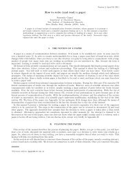
Figure 2.1: Comparison <strong>of</strong> numerical integration <strong>of</strong> φ with 1 st order perturbation<br />
result. The upper graph is a close up <strong>of</strong> the lower one near the horizon. The<br />
perturbation result is denoted by a dashed line. We chose α 1 , −α 2 = 1.7, Q 1 = 3,<br />
Q 2 = 3, δr = 2.3 × 10 −8 and c 1 in the range [− 1, 1]<br />
2 2<br />
. φ 0 = 0.<br />
28
2.2 Numerical Results<br />
Plot <strong>of</strong> Φ comparing numerical and 1 st order perturbation result Α 1 ⩵Α 2 ⩵3.1<br />
Φ<br />
0.3<br />
0.2<br />
0.1<br />
5 6 7 8<br />
r<br />
0.1<br />
Φ<br />
0.6<br />
0.4<br />
0.2<br />
50 100 150 200<br />
r<br />
0.2<br />
0.4<br />
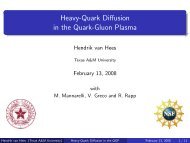
Figure 2.2: Comparison <strong>of</strong> numerical integration <strong>of</strong> φ with 1 st order perturbation<br />
result. The upper graph is a close up <strong>of</strong> the lower one near the horizon. The<br />
perturbation result is denoted by a dashed line. We chose α 1 , −α 2 = 3.1, Q 1 = 2,<br />
Q 2 = 3, δr = 2.9 × 10 −8 and c 1 is in the range [− 1, 1]<br />
2 2<br />
. φ 0 = 0.13.<br />
29
2.3 Exact Solutions<br />
where r i is the point at which we start the integration. c 1 refers to the asymptotic<br />
value for the scalar, eq.(2.42).<br />
In figs. (2.1,2.2) we compare the numerical and 1 st order correction. The<br />
numerical and perturbation results are denoted by solid and dashed lines respectively.<br />
We see good agreement even for large r. As expected, as we increase the<br />
asymptotic value <strong>of</strong> φ, which was the small parameter in our perturbation series,<br />
the agreement decreases.<br />
Note also that the resulting solutions turn out to be singularity free and<br />
asymptotically flat for a wide range <strong>of</strong> initial conditions. In this simple example<br />
there is only one critical point, eq.(2.33). This however does not guarantee that<br />
the attractor mechanism works. It could have been for example that as the<br />
asymptotic value <strong>of</strong> the scalar becomes significantly different from the attractor<br />
value no double-zero horizon black hole is allowed and instead one obtains a<br />
singularity. We have found no evidence for this. Instead, at least for the range <strong>of</strong><br />
asymptotic values for the scalars we scanned in the numerical work, we find that<br />
the attractor mechanism works with attractor value, eq.(2.33).<br />
It will be interesting to analyse this more completely, extending this work to<br />
cases where the effective potential is more complicated and several critical points<br />
are allowed. This should lead to multiple basins <strong>of</strong> attraction as has already been<br />
discussed in the supersymmetric context in e.g., [15, 16].<br />
2.3 Exact Solutions<br />
In certain cases the equation <strong>of</strong> motion can be solved exactly [17]. In this section,<br />
we shall look at some solvable cases and confirm that the extremal solutions<br />
display attractor behaviour. In particular, we shall work in 4 dimensions with<br />
one scalar and two gauge fields, taking V eff to be given by eq.(2.32),<br />
V eff = e α1φ (Q 1 ) 2 + e α2φ (Q 2 ) 2 . (2.68)<br />
We find that at the horizon the scalar field relaxes to the attractor value (2.33)<br />
e (α 1−α 2 )φ 0<br />
= − α 2Q 2 2<br />
α 1 Q 2 1<br />
(2.69)<br />
30
2.3 Exact Solutions<br />
which is the critical point <strong>of</strong> V eff and independent <strong>of</strong> the asymptotic value, φ ∞ .<br />
Furthermore, the horizon area is also independent <strong>of</strong> φ ∞ and, as predicted in<br />
section 2.1.2, it is proportional to the effective potential evaluated at the attractor<br />
point. It is given by<br />
Area = 4πb 2 H = 4πV eff(φ 0 ) (2.70)<br />
= 4π♠(Q 1 ) 2 −α 2<br />
α 1 −α 2 (Q 2 ) 2 α 1<br />
α 1 −α 2 (2.71)<br />
where<br />
♠ =<br />
( ) α 1 ( ) −α 2<br />
− α α<br />
2 1 −α 2<br />
α 1<br />
+ − α α<br />
2 1 −α 2<br />
α 1<br />
(2.72)<br />
is a numerical factor. It is worth noting that when α 1 = −α 2 , one just has<br />
1<br />
4 Area = 2π|Q 1Q 2 | (2.73)<br />
Interestingly, the solvable cases we know correspond to γ = 1, 2, 3 where γ<br />
is given by (2.43). The known solutions for γ = 1, 2 are discussed in [17] and<br />
references therein (although they fixed φ ∞ = 0). We found a solution for γ = 3<br />
and it appears as though one can find exact solutions as long as γ is a positive<br />
integer. Details <strong>of</strong> how these solutions are obtained can be found in the references<br />
and section 2.10.<br />
For the cases we consider, the extremal solutions can be written in the following<br />
form<br />
e (α 1−α 2 )φ<br />
=<br />
(<br />
− α ) ( ) 2 ( ) −<br />
1<br />
2 Q2 f2 2 α 1α 2<br />
(2.74)<br />
α 1 Q 1 f 1<br />
b 2 = ♠ ( (Q 1 f 1 ) −α 2<br />
(Q 2 f 2 ) α 1 ) 2<br />
α 1 −α 2 (2.75)<br />
a 2 = ρ 2 /b 2 (2.76)<br />
where ρ = r − r H and the f i are polynomials in ρ to some fractional power. In<br />
general the f i depend on φ ∞ but they have the property<br />
f i | Horizon = 1. (2.77)<br />
Substituting (2.77) into (2.74,2.75), one sees that that at the horizon the scalar<br />
field takes on the attractor value (2.69) and the horizon area is given by (2.71).<br />
31
2.3 Exact Solutions<br />
Φ log Q 2 Q 1 <br />
Φr for various values <strong>of</strong> Φ ∞ extremal bh, Α⩵2<br />
0.5<br />
0.25<br />
2 4 6 8 10<br />
r<br />
<br />
M<br />
0.25<br />
0.5<br />
0.75<br />
1<br />
Figure 2.3: Attractor behaviour for the case γ = 1; α 1 , −α 2 = 2<br />
Φ logQ 2 Q 1 <br />
<br />
3<br />
2<br />
<br />
Φr for various values <strong>of</strong> Φ ∞ extremal bh, Α⩵2 3 <br />
0.2<br />
2 4 6 8 10<br />
r<br />
<br />
M<br />
0.2<br />
0.4<br />
0.6<br />
Figure 2.4: Attractor behaviour for the case γ = 2; α 1 , −α 2 = 2 √ 3<br />
32
2.3 Exact Solutions<br />
Notice that, when α = |α i |, (2.74,2.75) simplify to<br />
e αφ = |Q ( ) 1<br />
2| f2 4 α2 (2.78)<br />
|Q 1 | f 1<br />
b 2 = 2|Q 1 ||Q 2 | (f 1 f 2 ) (2.79)<br />
2.3.1 Explicit Form <strong>of</strong> the f i<br />
In this section we present the form <strong>of</strong> the functions f i mainly to show that,<br />
although they depend on φ ∞ in a non trivial way, they all satisfy (2.77) which<br />
ensures that the attractor mechanism works. It is convenient to define<br />
¯Q 2 i = eα iφ ∞<br />
Q 2 i (no summation) (2.80)<br />
which are the effective U(1) charges as seen by an asymptotic observer. For the<br />
simplest case, γ = 1, we have<br />
f i = 1 +<br />
Taking γ = 2 and α 1 = −α 2 = 2 √ 3 one finds<br />
( )<br />
¯Q−1 i |α i |(4 + αi 2 1 )− 2<br />
ρ (2.81)<br />
f i =<br />
(1 + ( ¯Q 1 ¯Q2 ) − 2 2<br />
3 (<br />
3 ¯Q 1 + ¯Q<br />
2<br />
3<br />
2 ) 1 2 ρ +<br />
1<br />
( ¯Q<br />
) 1<br />
2 i ¯Q1 ¯Q2 ) − 2 2<br />
3 ρ<br />
2<br />
(2.82)<br />
Finally for γ = 3 and α 1 = 4 , α 2 = −6 we have<br />
f 1 = ( 1 − 6a 2 ρ + 12a 2 2 ρ2 − 6a 0 ρ 3) 1 3<br />
(2.83)<br />
f 2 = ( 1 − 24<br />
3 a 2ρ + 24a 2 ρ 2 − (48a 3 2 − 12a 0)ρ 3 + ( 48a 4 2 − 24a 0a 2<br />
)<br />
ρ<br />
4 ) 1 4<br />
(2.84)<br />
where a 0 and a 2 are non-trivial functions <strong>of</strong> ¯Qi . Further details are discussed<br />
in section 2.8 and section 2.10. The scalar field solutions for γ = 1 and 2 are<br />
illustrated in figs. 2.3 and 2.4 respectively.<br />
2.3.2 Supersymmetry and the Exact Solutions<br />
As mentioned above, the first two cases (γ = 1, 2) have been extensively studied<br />
in the literature.<br />
33
2.4 General Higher Dimensional Analysis<br />
The SUSY <strong>of</strong> the extremal α 1 = −α 2 = 2 solution is discussed in [18]. They<br />
show that it is supersymmetric in the context <strong>of</strong> N = 4 SUGRA. It saturates the<br />
BPS bound and preserves 1 <strong>of</strong> the supersymmetry - ie. it has N = 1 SUSY. There<br />
4<br />
are BPS black-holes in this context which carry only one U(1) charge and preserve<br />
1<br />
2<br />
<strong>of</strong> the supersymmetry. The non-extremal blackholes are <strong>of</strong> course non-BPS.<br />
On the other hand, the extremal α 1 = −α 2 = 2 √ 3 blackhole is non-BPS<br />
[19]. It arises in the context <strong>of</strong> dimensionally reduced 5D Kaluza-Klein gravity<br />
[20] and is embeddable in N = 2 SUGRA. There however are BPS black-holes in<br />
this context which carry only one U(1) charge and once again preserve 1 <strong>of</strong> the<br />
2<br />
supersymmetry [21].<br />
We have not investigated the supersymmetry <strong>of</strong> the γ = 3 solution, we expect<br />
that it is not a BPS solution in a supersymmetric theory.<br />
2.4 General Higher Dimensional Analysis<br />
2.4.1 The Set-Up<br />
It is straightforward to generalise our results above to higher dimensions. We<br />
start with an action <strong>of</strong> the form,<br />
S = 1 κ 2 ∫<br />
d d x √ −G(R − 2(∂φ i ) 2 − f ab (φ i )F a F b ) (2.85)<br />
Here the field strengths, F a are (d − 2) forms which are magnetic dual to 2-form<br />
fields.<br />
We will be interested in solution which preserve a SO(d − 2) rotation symmetry.<br />
Assuming all quantities to be function <strong>of</strong> r, and taking the charges to be<br />
purely magnetic, the ansatz for the metric and gauge fields is 1<br />
ds 2 = −a(r) 2 dt 2 + a(r) −2 dr 2 + b(r) 2 dΩ 2 d−2 (2.86)<br />
F a = Q a sin d−3 θ sin d−4 φ · · · dθ ∧ dφ ∧ · · · (2.87)<br />
1 Black hole which carry both electric and magnetic charges do not have an SO(d − 2)<br />
symmetry for general d and we only consider the magnetically charged case here. The analogue<br />
<strong>of</strong> the two-form in 4 dimensions is the d/2 form in d dimensions. In this case one can turn on<br />
both electric and magnetic charges consistent with SO(d/2) symmetry. We leave a discussion<br />
<strong>of</strong> this case and the more general case <strong>of</strong> p-forms in d dimensions for the future.<br />
34
2.4 General Higher Dimensional Analysis<br />
˜F a = Q a sin d−3 θ sin d−4 φ · · · dθ ∧ dφ ∧ · · · (2.88)<br />
The equation <strong>of</strong> motion for the scalars is<br />
∂ r (a 2 b d−2 ∂ r φ i ) = (d − 2)!∂ iV eff<br />
4b d−2 . (2.89)<br />
Here V eff , the effective potential for the scalars, is given by<br />
V eff = f ab (φ i )Q a Q b . (2.90)<br />
From the (R rr − Gtt<br />
G rr R tt ) component <strong>of</strong> the Einstein equation we get,<br />
∑<br />
i<br />
(φ ′ i )2 = − (d − 2)b′′ (r)<br />
2b(r)<br />
The R rr component gives the constraint,<br />
. (2.91)<br />
−(d − 2){(d − 3) − ab ′ (2a ′ b + (d − 3)ab ′ )} = 2φ ′2<br />
i a2 b 2 − (d−2)!<br />
b 2(d−3) V eff (φ i ) (2.92)<br />
In the analysis below we will use eq.(2.89) to solve for the scalars and then<br />
eq.(2.91) to solve for b. The constraint eq.(2.92) will be used in solving for a<br />
along with one extra relation, R tt = (d − 3) a2<br />
b 2 R θθ , as is explained in section 2.11.<br />
These equations (aside from the constraint) can be derived from a one-dimensional<br />
action<br />
S = 1 κ 2 ∫<br />
dr<br />
(<br />
(d − 3)(d − 2)b d−4 (1 + a 2 b ′2 ) + (d − 2)b d−3 (a 2 ) ′ b ′<br />
−2a 2 b d−2 (∂ r φ) 2 − (d−2)!<br />
b d−2 V eff<br />
) (2.93)<br />
As the analysis below shows if the potential has a critical point at φ i = φ i0<br />
and all the eigenvalues <strong>of</strong> the second derivative matrix ∂ ij V (φ i0 ) are positive then<br />
the attractor mechanism works in higher dimensions as well.<br />
2.4.2 Zeroth and First Order Analysis<br />
Our starting point is the case where the scalars take asymptotic values equal to<br />
their critical value, φ i = φ i0 . In this case it is consistent to set the scalars to be<br />
35
2.4 General Higher Dimensional Analysis<br />
a constant, independent <strong>of</strong> r. The extremal Reissner Nordstrom black hole in d<br />
dimensions is then a solution <strong>of</strong> the resulting equations. This takes the form,<br />
)<br />
a 0 (r) =<br />
(1 − rd−3 H<br />
b<br />
r d−3 0 (r) = r (2.94)<br />
where r H is the horizon radius. From the eq.(2.92) evaluated at r H we obtain the<br />
relation,<br />
r 2(d−3)<br />
H<br />
= (d − 4)!V eff (φ i0 ) (2.95)<br />
Thus the area <strong>of</strong> the horizon and the entropy <strong>of</strong> the black hole are determined by<br />
the value <strong>of</strong> V eff (φ i0 ), as in the four-dimensional case.<br />
Now, let us set up the first order perturbation in the scalar fields,<br />
The first order correction satisfies,<br />
φ i = φ i0 + ɛφ i1 (2.96)<br />
∂ r (a 2 0b d−2<br />
0 ∂ r φ i1 ) = β2 i<br />
b d−2 φ i1 (2.97)<br />
where, βi<br />
2 is the eigenvalue <strong>of</strong> the second derivative matrix (d−2)! ∂<br />
4 ij V eff (φ i0 ) corresponding<br />
to the mode φ i . This equation has two solutions. If βi<br />
2 > 0 one <strong>of</strong><br />
these solutions blows up while the other is well defined and goes to zero at the<br />
horizon. This second solution is the one we will be interested in. It is given by,<br />
φ i1 = c i1 (1 − r d−3<br />
H /rd−3 ) γ i<br />
(2.98)<br />
where γ is given by<br />
γ i = 1 2<br />
( √<br />
)<br />
−1 + 1 + 4βi 2r6−2d<br />
H /(d − 3)2<br />
(2.99)<br />
2.4.2.1 Second order calculations (Effects <strong>of</strong> backreaction)<br />
The first order perturbation in the scalars gives rise to a second order correction<br />
for the metric components, a, b. We write,<br />
b(r) = b 0 (r) + ɛ 2 b 2 (r) (2.100)<br />
a(r) 2 = a 0 (r) 2 + ɛ 2 a 2 (r) (2.101)<br />
b(r) 2 = b 0 (r) 2 + 2ɛ 2 b 2 (r)b 0 (r) (2.102)<br />
36
2.4 General Higher Dimensional Analysis<br />
where a 0 , b 0 are given in eq.(2.94).<br />
From (2.91) one can solve for the second order perturbation b 2 (r). For simplicity<br />
we consider the case <strong>of</strong> a single scalar field, φ. The solution is given by<br />
double-integration form,<br />
∂r 2 b 2(r) = − 2<br />
(d − 2) r(∂ rφ 1 ) 2 = −c ′ 1 − r d−3<br />
1<br />
r 2d−5 (rd−3 H<br />
r d−3<br />
c ′<br />
⇒ b 2 (r) = d 1 r + d 2 −<br />
1r<br />
×<br />
2(d − 3)(d − 4)γ(2γ − 1)rH<br />
(<br />
2d<br />
−(d − 4)F [ 1<br />
d−4<br />
, 1 − 2γ, ; ( r H<br />
3−d d−3 r<br />
) d−3]<br />
) 2γ−2<br />
+(2γ − 1) ( )<br />
r Hr d−3<br />
F [ d−4<br />
2d−7<br />
, 1 − 2γ, ; ( r H<br />
d−3 d−3 r<br />
) d−3]) , (2.103)<br />
where c ′ 1 ≡ 2(d − 3)2 c 2 1 γ2 rH d /(d − 2), a positive definite constant, and F is Gauss’s<br />
Hypergeometric function. More generally, for several scalar fields, b 2 is obtained<br />
by summing over the contributions from each scalar field. The integration constants<br />
d 1 , d 2 , in eq.(2.103), can be fixed by coordinate transformations and requiring<br />
a double-zero horizon solution. We will choose coordinate so that the horizon<br />
is at r = r H , then as we will see shortly the extremality condition requires both<br />
d 1 , d 2 to vanish. As r → r H we have from eq.(2.103) that<br />
( r d−3 − r d−3 ) 2γ<br />
H<br />
b 2 (r) ∝ −<br />
(2.104)<br />
r d−3<br />
Since γ > 0, we see that b 2 vanishes at the horizon and thus the area and the<br />
entropy are uncorrected to second order. At large r, b 2 (r) ∝ O(r)+O(1)+O(r 7−2d )<br />
so asymptotic behaviour is consistent with asymptotic flatness <strong>of</strong> the solution.<br />
The analysis for a 2 is discussed in more detail in section 2.11. In the vicinity<br />
<strong>of</strong> the horizon one finds that there is one non-singular solution which goes<br />
like, a 2 (r) → C(r − r H ) (2γ+2) . This solution smoothly extends to r → ∞ and<br />
asymptotically, as r → ∞, goes to a constant which is consistent with asymptotic<br />
flatness.<br />
Thus we see that the backreaction <strong>of</strong> the metric is finite and well behaved. A<br />
double-zero horizon black hole continues to exist to second order in perturbation<br />
theory. It is asymptotically flat. The scalars in this solution at the horizon take<br />
their attractor values irrespective <strong>of</strong> their values at infinity..<br />
37
2.5 Attractor in AdS 4<br />
Finally, the analysis in principle can be extended to higher orders. Unlike four<br />
dimensions though an explicit solution for the higher order perturbations is not<br />
possible and we will not present such an higher order analysis here.<br />
We end with Fig 5. which illustrates the attractor behaviour in asymptotically<br />
flat 4 + 1 dimensional space. This figure has been obtained for the example,<br />
eq.(2.31, 2.32). The parameter δr is defined in eq.(2.67).<br />
Φ<br />
Numerical plot <strong>of</strong> Φr in 41 dimensions<br />
0.8<br />
0.6<br />
0.4<br />
0.2<br />
5 10 15 20<br />
r<br />
0.2<br />
0.4<br />
Α 1 ⩵Α 2 ⩵2. Q 1 ⩵ <br />
1<br />
<br />
2<br />
Q 2 ⩵ 2 Φ 0 ⩵0.346574 ∆r⩵7.07107 10 6<br />
Figure 2.5: Numerical plot <strong>of</strong> φ(r) with α 1 = −α 2 = 2 for the an extremal black<br />
hole in 4 + 1 dimensions displaying attractor behaviour.<br />
2.5 Attractor in AdS 4<br />
Next we turn to the case <strong>of</strong> Anti-de Sitter space in four dimensions. Our analysis<br />
will be completely analogous to the discussion above for the four and higher<br />
dimensional case and so we can afford to be somewhat brief below.<br />
The action in 4-dim. has the form<br />
S = 1 κ 2 ∫<br />
d 4 x √ −G(R − 2Λ − 2(∂φ i ) 2 − f ab (φ i )F a F b − 1 2 ˜f ab (φ i )ɛ µνρσ F a µν F b ρσ )<br />
(2.105)<br />
38
2.5 Attractor in AdS 4<br />
where Λ = −3/L 2 is the cosmological constant. For simplicity we will discuss<br />
the case with only one scalar field here.<br />
The generalisation to many scalars<br />
is immediate and along the lines <strong>of</strong> the discussion for asymptotically flat fourdimensional<br />
case. Also we take the coefficient <strong>of</strong> the scalar kinetic energy term<br />
to be field independent.<br />
For spherically symmetric solutions the metric takes the form, eq.(2.8). The<br />
field strengths are given by eq.(2.20). This gives rise to a one dimensional action<br />
S = 1 ∫ (<br />
dr 2 − (a 2 b 2 ) ′′ − 2a 2 bb ′′ − 2a 2 b 2 (∂<br />
κ 2 r φ) 2 − 2 V )<br />
eff<br />
+ 3b2 , (2.106)<br />
b 2 L 2<br />
where V eff is given by eq.(2.21). The equations <strong>of</strong> motion, which can be derived<br />
either from eq.(2.106) or directly from the action, eq.(2.105) are now given by,<br />
∂ r (a 2 b 2 ∂ r φ) = ∂ φV eff (φ)<br />
2b 2 (2.107)<br />
b ′′<br />
b = −(∂ rφ) 2 , (2.108)<br />
which are unchanged from the flat four-dimensional case, and,<br />
(a 2 (r)b 2 (r)) ′′ = 2(1 − 2Λb 2 ), (2.109)<br />
− 1 + a 2 b ′2 b<br />
+ a2′ 2′<br />
= −1<br />
2 b (V eff(φ)) + a 2 b 2 (∂ 2 r φ) 2 + 3b2<br />
L , (2.110)<br />
2<br />
where the last equation is the first order constraint.<br />
2.5.1 Zeroth and First Order Analysis for V<br />
The zeroth order solution is obtained by taking the asymptotic values <strong>of</strong> the<br />
scalar field to be its critical values, φ 0 such that ∂ i V eff (φ 0 ) = 0.<br />
The resulting metric is now the extremal Reissner Nordstrom black hole in<br />
AdS space, [22], given by,<br />
a 0 (r) 2 = (r − r H) 2 (L 2 + 3r 2 H + 2r Hr + r 2 )<br />
L 2 r 2 (2.111)<br />
b 0 (r) = r (2.112)<br />
39
2.5 Attractor in AdS 4<br />
The horizon radius r H is given by evaluating the constraint eq.(2.110) at the<br />
horizon,<br />
(L 2 r 2 H + 2r4 H )<br />
L 2 = V eff (φ 0 ).<br />
The first order perturbation for the scalar satisfies the equation,<br />
(2.113)<br />
where,<br />
∂ r (a 2 0b 2 0∂ r φ 1 ) = β2<br />
b 2 φ 1 (2.114)<br />
β 2 = 1 2 ∂2 φV eff (φ 0 ). (2.115)<br />
This is difficult to solve explicitly.<br />
In the vicinity <strong>of</strong> the horizon the two solutions are given by<br />
φ 1 = C ± (r − r H ) t ±<br />
(2.116)<br />
If V ′′<br />
eff (φ 0) > 0 one <strong>of</strong> the two solutions vanishes at the horizon. We are interested<br />
in this solution. It corresponds to the choice,<br />
where,<br />
φ 1 = C(r − r H ) γ , (2.117)<br />
γ =<br />
√<br />
1 + 4β2<br />
δrH<br />
2<br />
2<br />
− 1<br />
, (2.118)<br />
and, δ = (L2 +6rH 2 ) . As discussed in the section 2.12 this solution behaves at r → ∞<br />
L 2<br />
as φ 1 → C 1 + C 2 /r 3 . Also, all other values <strong>of</strong> r, besides the horizon and ∞, are<br />
ordinary points <strong>of</strong> the second order equation eq.(2.114). All this establishes that<br />
there is one well-behaved solution for the first order scalar perturbation. In the<br />
vicinity <strong>of</strong> the horizon it takes the form eq.(2.116) with eq.(2.118), and vanishes<br />
at the horizon. It is non-singular everywhere between the horizon and infinity<br />
and it goes to a constant asymptotically at r → ∞.<br />
We consider metric corrections next. These arise at second order. We define<br />
the second order perturbations as in eq.(2.45). The equation for b 2 from the<br />
second order terms in eq.(2.108) takes the form,<br />
b ′′<br />
2 = −r(φ′ 1 (r))2 , (2.119)<br />
40
2.5 Attractor in AdS 4<br />
and can be solved to give,<br />
∫<br />
b 2 (r) = − [r(φ<br />
∫r ′ 1 (r))2 ] (2.120)<br />
H r H<br />
We fix the integration constants by taking take the lower limit <strong>of</strong> both integrals<br />
to be the horizon. We will see that this choice gives rise to an double-zero horizon<br />
solution. Since φ 1 is well behaved for all r H ≤ r ≤ ∞ the integrand above is well<br />
behaved as well. Using eq.(2.116) we find that in the near horizon region<br />
b 2 ∼ (r − r H ) (2γ) (2.121)<br />
At r → ∞ using the fact that φ 1 → C 1 + C 2 /r 3 we find<br />
b 2 ∼ D 1 r + D 2 + D 3 /r 6 . (2.122)<br />
This is consistent with an asymptotically AdS solution.<br />
Finally we turn to a 2 . As we show in section 2.12 a solution can be found for<br />
a 2 with the following properties. In the vicinity <strong>of</strong> the horizon it goes like,<br />
a 2 ∝ (r − r H ) (2γ+2) , (2.123)<br />
and vanishes faster than a double-zero. As r → ∞, a 2 → d 1 r and grows more<br />
slowly than a 2 0 . And for r H < r < ∞ it is well-behaved and non-singular.<br />
This establishes that after including the backreaction <strong>of</strong> the metric we have<br />
a non-singular, double-zero horizon black hole which is asymptotically AdS. The<br />
scalar takes a fixed value at the horizon <strong>of</strong> the black hole and the entropy <strong>of</strong> the<br />
black hole is unchanged as the asymptotic value <strong>of</strong> the scalar is varied.<br />
Let us end with two remarks. In the AdS case one can hope that there is a<br />
dual description for the attractor phenomenon. Since the asymptotic value <strong>of</strong> the<br />
scalar is changing we are turning on a operator in the dual theory with a varying<br />
value for the coupling constant. The fact that the entropy, for fixed charge, does<br />
not change means that the number <strong>of</strong> ground states in the resulting family <strong>of</strong> dual<br />
theories is the same. This would be worth understanding in the dual description<br />
better. Finally, we expect this analysis to generalise in a straightforward manner<br />
to the AdS space in higher dimensions as well.<br />
Fig. 6 illustrates the attractor mechanism in asymptotically AdS 4 space. This<br />
Figure is for the example, eq.(2.31, 2.32). The cosmological constant is taken to<br />
be, Λ = −2.91723, in κ = 1 units.<br />
41
2.6 Additional Comments<br />
Φ<br />
Numerical plot <strong>of</strong> Φr in AdS 4<br />
0.6<br />
0.4<br />
0.2<br />
0.2<br />
5 10 15 20<br />
Α 1 ⩵Α 2 ⩵2. Q 1 ⩵ <br />
1<br />
<br />
2<br />
Q 2 ⩵ 2 Φ 0 ⩵0.346574 ∆r⩵0.0150842 ⩵2.91723<br />
r<br />
Figure 2.6: Numerical plot <strong>of</strong> φ(r) with α 1 = −α 2 = 2 for the an extremal black<br />
hole in AdS 4 displaying attractor behaviour.<br />
2.6 Additional Comments<br />
The theories we considered in the discussion <strong>of</strong> asymptotically flat space-times<br />
and AdS spacetimes have no potential for the scalars. We comment on this further<br />
here.<br />
Let us consider a theory with N = 1 supersymmetry containing chiral superfields<br />
whose lowest component scalars are,<br />
S i = φ i + ia i (2.124)<br />
We take these scalars to be uncharged under the gauge symmetries. These can<br />
be coupled to the superfields Wα a by a coupling<br />
∫<br />
L gaugekinetic = d 2 θf ab (S i )Wα a W α b (2.125)<br />
Such a coupling reproduces the gauge kinetic energy terms in and eq.(2.105),<br />
eq.(2.106), (we now include both φ i , a i in the set <strong>of</strong> scalar fields which we denoted<br />
by φ i in the previous sections).<br />
42
2.6 Additional Comments<br />
An additional potential for the scalars would arise due to F-term contributions<br />
from a superpotential. If the superpotential is absent we get the required feature<br />
<strong>of</strong> no potential for these scalar. Setting the superpotential to be zero is at least<br />
technically natural due to its non-renormalisability.<br />
In a theory with no supersymmetry there is no natural way to suppress a<br />
potential for the scalars and it would arise due to quantum effects even if it is<br />
absent at tree-level. In this case we have no good argument for not including a<br />
potential for the scalar and our analysis is more in the nature <strong>of</strong> a mathematical<br />
investigation.<br />
The absence <strong>of</strong> a potential is important also for avoiding no-hair theorems<br />
which <strong>of</strong>ten forbid any scalar fields from being excited in black hole backgrounds<br />
[? ]. In the presence <strong>of</strong> a mass m in asymptotically flat four dimensional space<br />
the two solutions for first order perturbation at asymptotic infinity go like,<br />
φ ∼ C 1 e mr /r, φ ∼ C 2 e −mr /r. (2.126)<br />
We see that one <strong>of</strong> the solutions blows up as r → ∞. Since one solution to the<br />
equation <strong>of</strong> motion also blows up in the vicinity <strong>of</strong> the horizon, as discussed in<br />
section 2, there will generically be no non-singular solution in first order perturbation<br />
theory. This argument is a simple-minded way <strong>of</strong> understanding the absence<br />
<strong>of</strong> scalar hair for extremal black holes under discussion here. In the absence <strong>of</strong><br />
mass terms, as was discussed in section 2, the two solutions at asymptotic infinity<br />
go like φ ∼ const and φ ∼ 1/r respectively and are both acceptable. This is why<br />
one can turn on scalar hair. The possibility <strong>of</strong> scalar hair for a massless scalar<br />
is <strong>of</strong> course well known. See [23], [17], for some early examples <strong>of</strong> solutions with<br />
scalar hair, [24, 25, 26, 27], for theorems on uniqueness in the presence <strong>of</strong> such<br />
hair, and [28] for a discussion <strong>of</strong> resulting thermodynamics.<br />
In asymptotic AdS space the analysis is different. Now the (mass) 2 for scalars<br />
can be negative as long as it is bigger than the BF bound. In this case both solutions<br />
at asymptotic infinity decay and are acceptable. Thus, as for the massless<br />
case, it should be possible to turn on scalar fields even in the presence <strong>of</strong> these<br />
mass terms and study the resulting black holes solutions. Unfortunately, the resulting<br />
equations are quite intractable. For small (mass) 2 we expect the attractor<br />
mechanism to continue to work.<br />
43
2.7 Asymptotic de Sitter Space<br />
If the (mass) 2 is positive one <strong>of</strong> the solutions in the asymptotic region blows<br />
up and the situation is analogous to the case <strong>of</strong> a massive scalar in flat space<br />
discussed above. In this case one could work with AdS space which is cut <strong>of</strong>f at<br />
large r (in the infrared) and study the attractor phenomenon. Alternatively, after<br />
incorporating back reaction, one might get a non-singular geometry which departs<br />
from AdS in the IR and then analyse black holes in this resulting geometry. In<br />
the dual field theory a positive (mass) 2 corresponds to an irrelevant operator.<br />
The growing mode in the bulk is the non-normalisable one and corresponds to<br />
turning on a operator in the dual theory which grows in the UV. Cutting <strong>of</strong>f<br />
AdS space means working with a cut-<strong>of</strong>f effective theory. Incorporating the backreaction<br />
means finding a UV completion <strong>of</strong> the cut-<strong>of</strong>f theory. And the attractor<br />
mechanism means that the number <strong>of</strong> ground states at fixed charge is the same<br />
regardless <strong>of</strong> the value <strong>of</strong> the coupling constant for this operator.<br />
2.7 Asymptotic de Sitter Space<br />
In de Sitter space the simplest way to obtain a double-zero horizon is to take<br />
a Schwarzschild black hole and adjust the mass so that the de Sitter horizon<br />
and the Schwarzschild horizon coincide. The resulting black hole is the extreme<br />
Schwarzschild-de Sitter spacetime [29]. We will analyse the attractor behaviour<br />
<strong>of</strong> this black hole below.<br />
The analysis simplifies in 5-dimensions and we will<br />
consider that case, a similar analysis can be carried out in other dimensions as<br />
well. Since no charges are needed we set all the gauge fields to zero and work<br />
only with a theory <strong>of</strong> gravity and scalars. Of course by turning on gauge charges<br />
one can get other double-zero horizon black holes in dS, their analysis is left for<br />
the future.<br />
We start with the action <strong>of</strong> the form,<br />
S = 1 κ 2 ∫<br />
d 5 x √ −G(R − 2(∂φ) 2 − V (φ)) (2.127)<br />
Notice that the action now includes a potential for the scalar, V (φ), it will play<br />
the role <strong>of</strong> V eff in our discussion <strong>of</strong> asymptotic flat space and AdS space. The<br />
required conditions for an attractor in the dS case will be stated in terms <strong>of</strong> V . A<br />
44
2.7 Asymptotic de Sitter Space<br />
concrete example <strong>of</strong> a potential meeting the required conditions will be given at<br />
the end <strong>of</strong> the section. For simplicity we have taken only one scalar, the analysis<br />
is easily extended for additional scalars.<br />
The first condition on V is that it has a critical point, V ′ (φ 0 ) = 0. We will<br />
also require that V (φ 0 ) > 0. Now if the asymptotic value <strong>of</strong> the scalar is equal to<br />
its critical value, φ 0 , we can consistently set it to this value for all times t. The<br />
resulting equations have a extremal black hole solution mentioned above. This<br />
takes the form<br />
t 2<br />
ds 2 = −<br />
(t 2 /L − L/2) 2 dt2 + (t2 /L − L/2) 2<br />
dr 2 + t 2 dΩ 2<br />
t 2 3 (2.128)<br />
Notice that it is explicitly time dependent. L is a length related to V (φ 0 ) by ,<br />
V (φ 0 ) = 20<br />
L 2 . And t = ± L √<br />
2<br />
is the location <strong>of</strong> the double-zero horizon. A suitable<br />
near-horizon limit <strong>of</strong> this geometry is called the Nariai solution, [30].<br />
2.7.1 Perturbation Theory<br />
Starting from this solution we vary the asymptotic value <strong>of</strong> the scalar. We take<br />
the boundary at t → −∞ as the initial data slice and investigate what happens<br />
when the scalar takes a value different from φ 0 as t → −∞. Our discussion<br />
will involve part <strong>of</strong> the space-time, covered by the coordinates in eq.(2.128), with<br />
−∞ ≤ t ≤ t H = − √ L 2<br />
. We carry out the analysis in perturbation theory below.<br />
Define the first order perturbation for the scalar by,<br />
This satisfies the equation,<br />
φ = φ 0 + ɛφ 1<br />
∂ t (a 2 0 b3 0 ∂ tφ 1 ) = b3<br />
4 V ′′ (φ 0 )φ 1 (2.129)<br />
where a 0 = (t2 /L−L/2)<br />
, b<br />
t 0 = t. This equation is difficult to solve in general.<br />
In the vicinity <strong>of</strong> the horizon t = t H , we have two solutions which go like,<br />
φ 1 = C ± (t − t H ) −1+ √<br />
1+κ 2<br />
2 (2.130)<br />
where<br />
κ 2 = − 1 4 V ′′ (φ 0 ) (2.131)<br />
45
2.7 Asymptotic de Sitter Space<br />
We see that one <strong>of</strong> the two solutions in eq.(2.130) is non-divergent and in fact<br />
vanishes at the horizon if<br />
V ′′ (φ 0 ) < 0. (2.132)<br />
We will henceforth assume that the potential meets this condition. Notice this<br />
condition has a sign opposite to what was obtained for the asymptotically flat or<br />
AdS cases. This reversal <strong>of</strong> sign is due to the exchange <strong>of</strong> space and time in the<br />
dS case.<br />
In the vicinity <strong>of</strong> t → −∞ there are two solutions to eq.(2.129) which go like,<br />
φ 1 = ˜C ± |t| p ±<br />
(2.133)<br />
where<br />
p ± = 2(−1 ± √ 1 + κ 2 /4). (2.134)<br />
If the potential meets the condition, eq.(2.132) then κ 2 > 0 and we see that one<br />
<strong>of</strong> the modes blows up at t → −∞.<br />
2.7.2 Some Speculative Remarks<br />
In view <strong>of</strong> the diverging mode at large |t| one needs to work with a cut<strong>of</strong>f version<br />
<strong>of</strong> dS space 1 . With such a cut<strong>of</strong>f at large negative t we see that there is a<br />
one parameter family <strong>of</strong> solutions in which the scalar takes a fixed value at the<br />
horizon. The one parameter family is obtained by starting with the appropriate<br />
linear combination <strong>of</strong> the two solutions at t → −∞ which match to the well<br />
behaved solution in the vicinity <strong>of</strong> the horizon. While we will not discuss the<br />
metric perturbations and scalar perturbations at second order these too have a<br />
non-singular solution which preserves the double-zero nature <strong>of</strong> the horizon. The<br />
metric perturbations also grow at the boundary in response to the growing scalar<br />
mode and again the cut-<strong>of</strong>f is necessary to regulate this growth. This suggests<br />
that in the cut-<strong>of</strong>f version <strong>of</strong> dS space one has an attractor phenomenon. Whether<br />
such a cut-<strong>of</strong>f makes physical sense and can be implemented appropriately are<br />
question we will not explore further here.<br />
1 This is related to some comments made in the previous section in the positive (mass) 2<br />
case in AdS space.<br />
46
2.8 Non-Extremal = Unattractive<br />
One intriguing possibility is that quantum effects implement such a cut-<strong>of</strong>f and<br />
cure the infra-red divergence. The condition on the potential eq.(2.132) means<br />
that the scalar has a negative (mass) 2 and is tachyonic. In dS space we know<br />
that a tachyonic scalar can have its behaviour drastically altered due to quantum<br />
effects if it has a (mass) 2 < H 2 where H is the Hubble scale <strong>of</strong> dS space. This<br />
can certainly be arranged consistent with the other conditions on the potential<br />
as we will see below. In this case the tachyon can be prevented from “falling<br />
down” at large |t| due to quantum effects and the infrared divergences can be<br />
arrested by the finite temperature fluctuations <strong>of</strong> dS space. It is unclear though<br />
if any version <strong>of</strong> <strong>of</strong> the attractor phenomenon survives once these quantum effects<br />
became important.<br />
We end by discussing one example <strong>of</strong> a potential which meets the various<br />
conditions imposed above. Consider a potential for the scalar,<br />
V = Λ 1 e α 1φ + Λ 2 e α 2φ . (2.135)<br />
We require that it has a critical point at φ = φ 0 and that the value <strong>of</strong> the potential<br />
at the critical point is positive. The critical point for the potential eq.(2.135) is<br />
at,<br />
Requiring that V (φ 0 ) > 0 tells us that<br />
( ) 1<br />
e φ α2 0<br />
Λ<br />
α 2 1 −α 2<br />
= −<br />
(2.136)<br />
α 1 Λ 1<br />
(<br />
V (φ 0 ) = Λ 2 e α 2φ 0<br />
1 − α )<br />
2<br />
> 0 (2.137)<br />
α 1<br />
Finally we need that V ′′ (φ 0 ) < 0 this leads to the condition,<br />
V ′′ (φ 0 ) = Λ 2 e α 2φ 0<br />
α 2 (α 2 − α 1 ) < 0 (2.138)<br />
These conditions can all be met by taking both α 1 , α 2 > 0, α 2 < α 1 , Λ 2 > 0 and<br />
Λ 1 < 0. In addition if α 2 α 1 ≫ 1 the resulting −(mass) 2 ≫ H 2 .<br />
2.8 Non-Extremal = Unattractive<br />
We end this chapter by examining the case <strong>of</strong> an non-extremal black hole which<br />
has a single-zero horizon. As we will see there is no attractor mechanism in this<br />
47
2.8 Non-Extremal = Unattractive<br />
case.<br />
Thus the existence <strong>of</strong> a double-zero horizon is crucial for the attractor<br />
mechanism to work.<br />
Our starting point is the four dimensional theory considered in section 2 with<br />
action eq.(2.17). For simplicity we consider only one scalar field. We again start<br />
by consistently setting this scalar equal to its critical value, φ 0 , for all values <strong>of</strong> r,<br />
but now do not consider the extremal Reissner Nordstrom black hole. Instead we<br />
consider the non-extremal black hole which also solves the resulting equations.<br />
This is given by a metric <strong>of</strong> the form, eq.(2.8), with<br />
(<br />
a 2 (r) = 1 − r ) (<br />
+<br />
1 − r )<br />
−<br />
,<br />
r r<br />
b(r) = r (2.139)<br />
where r ± are not equal. We take r + > r − so that r + is the outer horizon which<br />
will be <strong>of</strong> interest to us.<br />
The first order perturbation <strong>of</strong> the scalar field satisfies the equation,<br />
∂ r (a 2 b 2 ∂ r φ i ) = V ′′<br />
eff (φ 0)<br />
4b 2 φ 1 (2.140)<br />
In the vicinity <strong>of</strong> the horizon r = r + this takes the form,<br />
∂ y (y∂ y φ 1 ) = αφ 1 (2.141)<br />
where α is a constant dependent on V ′′ (φ 0 ), r + , r − , and y ≡ r − r + .<br />
This equation has one non-singular solution which goes like,<br />
φ 1 = C 0 + C 1 y + · · · (2.142)<br />
where the ellipses indicate higher terms in the power series expansion <strong>of</strong> φ 1 around<br />
y = 0. The coefficients C 1 , C 2 , · · · are all determined in terms <strong>of</strong> C 0 which can<br />
take any value. Thus we see that unlike the case <strong>of</strong> the double-horizon extremal<br />
black hole, here the solution which is well-behaved in the vicinity <strong>of</strong> the horizon<br />
does not vanish.<br />
Asymptotically, as r → ∞ both solutions to eq.(2.140) are well defined and<br />
go like 1/r, constant respectively. It is then straightforward to see that one can<br />
choose an appropriate linear combination <strong>of</strong> the two solutions at infinity and<br />
match to the solution, eq.(2.142) in the vicinity <strong>of</strong> the horizon. The important<br />
difference here is that the value <strong>of</strong> the constant C 0 in eq.(2.142) depends on the<br />
48
2.8 Non-Extremal = Unattractive<br />
asymptotic values <strong>of</strong> the scalar at infinity and therefore the value <strong>of</strong> φ does not<br />
go to a fixed value at the horizon. The metric perturbations sourced by the scalar<br />
perturbation can also be analysed and are non-singular. In summary, we find a<br />
family <strong>of</strong> non-singular black hole solutions for which the scalar field takes varying<br />
values at infinity. The crucial difference is that here the scalar takes a value at<br />
the horizon which depends on its value at asymptotic infinity. The entropy and<br />
mass for these solutions also depends on the asymptotic value <strong>of</strong> the scalar 1 .<br />
It is also worth examining this issue in a non-extremal black holes for an<br />
exactly solvable case.<br />
If we consider the case |α i | = 2, section 2.3, the non-extremal solution takes<br />
on a relatively simple form. It can be written[18]<br />
(r + Σ)<br />
2φ∞<br />
exp(2φ) = e<br />
(r − Σ)<br />
a 2 = (r − r +)(r − r − )<br />
(r 2 − Σ 2 )<br />
b 2 = (r 2 − Σ 2 )<br />
(2.143)<br />
where 2 r ± = M ± r 0 r 0 =<br />
√<br />
M 2 + Σ 2 − ¯Q 2 2 − ¯Q 2 1 . (2.144)<br />
and the Hamiltonian constraint becomes<br />
Σ 2 + M 2 − ¯Q 2 1 − ¯Q 2 2 = 1 4 (r + − r − ) 2 . (2.145)<br />
The scalar charge, Σ, defined by φ ∼ φ ∞ + Σ , is not an independent parameter.<br />
r<br />
It is given by<br />
Σ = ¯Q 2 2 − ¯Q 2 1<br />
2M . (2.146)<br />
There are horizons at r = r ± , the curvature singularity occurs at r = Σ and<br />
r 0 characterises the deviation from extremality. We see that the non-extremal<br />
solution does not display attractor behaviour.<br />
Fig. 2.7 shows the behaviour <strong>of</strong> the scalar field 3 as we vary φ ∞ keeping M<br />
1 An intuitive argument was given in the introduction in support <strong>of</strong> the attractor mechanism.<br />
Namely, that the degeneracy <strong>of</strong> states cannot vary continuously. This argument only applies<br />
to the ground states. A non-extremal black hole corresponds to excited states. Changing the<br />
asymptotic values <strong>of</strong> the scalars also changes the total mass and hence the entropy in this case.<br />
2 The radial coordinate r in eq.(2.143) is related to our previous one by a constant shift.<br />
3 for α 1 = −α 2 = 2<br />
49
2.8 Non-Extremal = Unattractive<br />
and Q i fixed. The location <strong>of</strong> the horizon as a function <strong>of</strong> r depends on φ ∞ ,<br />
eq.(2.144). The horizon as a function <strong>of</strong> φ ∞ is denoted by the dotted line. The<br />
plot is terminated at the horizon.<br />
In contrast, for the extremal black hole,<br />
M = | ¯Q 2 | + | ¯Q 1 |<br />
√<br />
2<br />
Σ = | ¯Q 2 | − | ¯Q 1 |<br />
√<br />
2<br />
, (2.147)<br />
so (2.143) gives<br />
which is indeed the attractor value.<br />
e 2φ 0<br />
= e 2φ∞ M + Σ<br />
M − Σ = |Q 2|<br />
|Q 1 | , (2.148)<br />
Φ<br />
Φr for various values <strong>of</strong> Φ ∞<br />
nonextremal, M and Q i kept fixed, Α i ⩵2<br />
1<br />
0.5<br />
1 2 3 4 5 6<br />
r<br />
<br />
M<br />
0.5<br />
1<br />
Figure 2.7: Plot φ(r) with α 1 = −α 2 = 2 for the non-extremal black hole with<br />
M, Q i held fixed while varying φ ∞ . The dotted line denotes the outer horizon at<br />
which we terminate the plot. It is clearly unattractive.<br />
50
2.9 Perturbation Analysis<br />
2.9 Perturbation Analysis<br />
2.9.1 Mass<br />
Here, we first calculate the mass <strong>of</strong> the extremal black hole discussed in section<br />
2.2. From eq.(2.50), for large r, b 2 is given by,<br />
b 2 = cr + d (2.149)<br />
where<br />
c = − c2 1 γ<br />
2(2γ − 1)<br />
d = r Hc 2 1γ 2<br />
(2γ − 1)<br />
(2.150)<br />
(2.151)<br />
Now, we can easily write down the expression for a 2 using eq.(2.48). We choose<br />
coordinate y as introduced in eq.(2.51) such that at large r,<br />
r 2 + 2ɛ 2 (cr 2 + dr) = y 2 (2.152)<br />
1<br />
r<br />
= 1 y (1 + ɛ2 (c + d ))<br />
y<br />
(2.153)<br />
We use the extremality condition (2.54) to find,<br />
( ) r − rH<br />
a(r) =<br />
y<br />
(2.154)<br />
Using, eq.(2.149, 2.154) one finds that asymptotically, as r → ∞ the metric<br />
takes the form,<br />
ds 2 = −<br />
(<br />
1 − 2(r H + ɛ 2 (cr H + d))<br />
y<br />
)<br />
d˜t 2 +<br />
1<br />
(1 − 2(r H+ɛ 2 (cr H +d))<br />
) dy2 + y 2 dΩ 2<br />
y<br />
(2.155)<br />
where ˜t is obtained by rescaling t and dΩ 2 denotes the metric <strong>of</strong> S 2 . The mass<br />
M <strong>of</strong> the black hole is then given by the 1/y term in the g yy component <strong>of</strong> the<br />
metric. This gives,<br />
M = r H + ɛ 2 r Hc 2 1 γ . (2.156)<br />
2<br />
51
2.9 Perturbation Analysis<br />
2.9.2 Perturbation Series to All Orders<br />
Next we go on to discuss the perturbation series to all orders, Using (2.55) for b<br />
and (2.56) for φ in eq.(2.14)and eq.(2.62), we get,<br />
where<br />
∑<br />
i+jk<br />
V ik =<br />
k∑<br />
k−i<br />
k = − ∑<br />
b i φ ′ j φ′ k−i−j (2.157)<br />
b ′′<br />
i=0<br />
j=0<br />
2b j b k−i−j ((r − r H ) 2 φ ′ i )′ = Q 2 i eα iφ 0<br />
α i V ik (2.158)<br />
∑<br />
{n 1 ,n 2 ...n k }<br />
φ n 1<br />
1 φn 2<br />
2 . . . φn k<br />
k<br />
n 1 !n 2 ! . . . n k ! αn 1+n 2 +...+n k<br />
i . (2.159)<br />
(2.160)<br />
After substituting our ansatz (2.58)and (2.59), the above equations give,<br />
k(kγ − 1)d k = −γ ∑<br />
j(k − i − j)d i c j c k−i−j (2.161)<br />
and<br />
where S k and T k are given by<br />
and<br />
S k =<br />
i+j
2.10 Exact Analysis<br />
2.10 Exact Analysis<br />
Exact solutions can be found by writing the equations <strong>of</strong> motion as generalised<br />
Toda equations [31], which may, in certain special cases, be solved exactly [17] -<br />
we rederive this result in slightly different notation below. As noted in [32], in a<br />
marginally different context, the extremal solutions, are, in appropriate variables,<br />
polynomial solutions <strong>of</strong> the Toda equations. The polynomial solutions are much<br />
easier to find and are related to the functions f i mentioned in section 2.3. For<br />
ease <strong>of</strong> comparison we occasionally use notation similar to [32].<br />
2.10.1 New Variables<br />
To recast the equations <strong>of</strong> motion into a generalised Toda equation we define the<br />
following new variables<br />
u 1 = φ u 2 = log a z = log ab · = ∂ τ = a 2 b 2 ∂ r (2.167)<br />
In terms <strong>of</strong> r, τ is given by<br />
∫<br />
τ =<br />
( )<br />
dr<br />
a 2 b = 1 r − 2 (r + − r − ) log r+<br />
r − r −<br />
where r ± are the integration constants <strong>of</strong> (2.13). In general (2.13) implies<br />
Notice that<br />
(2.168)<br />
a 2 b 2 = (r − r + )(r − r − ). (2.169)<br />
τ → 0 as r → ∞ (2.170)<br />
τ → −∞ as r → r + (2.171)<br />
When we have a double-zero horizon, r H = r ± , τ takes the simple form<br />
τ −1 = −(r − r H ). (2.172)<br />
Since we are mainly interested in solutions with double-zero horizons, in what<br />
follows it will be convenient to work with a new radial coordinate, ρ, defined by<br />
which has the convenient property that ρ H = 0.<br />
ρ = −τ −1 . (2.173)<br />
53
2.10 Exact Analysis<br />
2.10.2 Equivalent Toda System<br />
In terms <strong>of</strong> these new variables the equations <strong>of</strong> motion become<br />
ü 1 = 1 2 α 1e 2u 2+α 1 u 1<br />
Q 2 1 + 1 2 α 2e 2u 2+α 2 u 1<br />
Q 2 2 (2.174)<br />
ü 2 = e 2u 2+α 1 u 1<br />
Q 2 1 + e2u 2+α 2 u 1<br />
Q 2 2 (2.175)<br />
¨z = e 2z (2.176)<br />
u˙<br />
2 1 + u˙<br />
2 2 − ż 2 + e 2z − e 2u 2+α 1 u 1<br />
Q 2 1 − e2u 2+α 2 u 1<br />
Q 2 2 = 0 (2.177)<br />
(2.176) decouples from the other equations and is equivalent to (2.13). Finally<br />
making the coordinate change<br />
where<br />
and<br />
X i = nij −1 u j + m −1<br />
ij log ( )<br />
(α 1 − α 2 )Q 2 j<br />
m ij =<br />
n −1 =<br />
( )<br />
2 −α2<br />
−2 α 1<br />
we obtain the generalised 2 body Toda equation<br />
together with<br />
∑<br />
ij<br />
(2.178)<br />
(2.179)<br />
1<br />
2 (α 1 − α 2 ) (4 + α iα j ) (2.180)<br />
Ẍ i = e m ijX j<br />
, (2.181)<br />
(<br />
1<br />
2Ẋim ij Ẋ j − e m ijX j<br />
)<br />
= (α 1 − α 2 )E (2.182)<br />
where E = 1 4 (r + − r − ) 2 . After solving the above, the original fields will be given<br />
by<br />
e (α 1−α 2 )φ<br />
= Q2 2<br />
e 1<br />
Q 2 2 (α 1X 1 +α 2 X 2 )<br />
1<br />
2<br />
(2.183)<br />
a 2 (X α<br />
= e 1 −α 1 +X 2 ) 2 /♦ (2.184)<br />
b 2 = (r − r + )(r − r − )/a 2 (2.185)<br />
where<br />
♦ = (α 1 − α 2 )Q 2 −α 2<br />
α 1 −α 2<br />
1 Q 2 α 1<br />
α 1 −α 2<br />
2 (2.186)<br />
54
2.10 Exact Analysis<br />
2.10.3 Solutions<br />
2.10.3.1 Case I: γ = 1 ⇔ α 1 α 2 = −4<br />
In this case, m ij is diagonal<br />
so the equations <strong>of</strong> motion decouple:<br />
m = diag(α 1 /2, −α 2 /2), (2.187)<br />
Ẍ i = e |α i |<br />
2 X i<br />
. (2.188)<br />
(2.188) has solutions<br />
X i = 2 (<br />
)<br />
|α i | log 4c 2 i<br />
|α i | sinh 2 (c i (τ − d i ))<br />
(2.189)<br />
The integration constants are fixed by imposing asymptotic boundary conditions<br />
and requiring that the solution is finite at the horizon. Letting<br />
in terms <strong>of</strong> φ and a we get<br />
F i = sinh(c i (τ − d i )) (2.190)<br />
e (α 1−α 2 )φ<br />
= Q2 2<br />
e 1<br />
Q 2 2 (α 1X 1 +α 2 X 2 )<br />
1<br />
(<br />
= − α ) ( ) 2<br />
2 Q2 F 2 c 1<br />
α 1 Q 1 F / 1 c 2<br />
a 2 2<br />
(X α<br />
= e 1 −α 1 +X 2 ) 2 ♦<br />
( ) −α 2 2 (<br />
c1 α 1 −α 2<br />
=<br />
Q 1 F 1<br />
) 2 c2<br />
Q 2 F 2<br />
/<br />
α<br />
α−˜α<br />
♠<br />
(2.191)<br />
As r → r + (ie. τ → −∞) the scalar field goes like<br />
e (α 1−α 2 )φ ∼ e 2(c 1−c 2 )τ<br />
(2.192)<br />
so we require<br />
c := c 1 = c 2 (2.193)<br />
for a finite solution at the horizon. Also at the horizon<br />
b 2 ∼ (r − r + )/a 2 ∼ e ((r +−r − )−2c)τ<br />
(2.194)<br />
55
2.10 Exact Analysis<br />
which necessitates<br />
(r + − r − ) = 2c (2.195)<br />
To find the extremal solutions we take the limit c → 0 which gives<br />
(<br />
e (α 1−α 2 )φ<br />
= − α )<br />
2 (Q2 f 2 ) 2<br />
α 1 (Q 1 f 1 ) 2 (2.196)<br />
b 2 = ♠ (Q 1 f 1 ) −2α 2<br />
α 1 −α 2 (Q 2 p 2 ) 2α 1<br />
α 1 −α 2 (2.197)<br />
a 2 = ρ 2 /b 2 (2.198)<br />
where<br />
f i = 1 + d i ρ. (2.199)<br />
Requiring φ → φ ∞ and a → 1 as r → ∞ fixes<br />
√<br />
d i = ¯Q<br />
−1 |α i |<br />
i (2.200)<br />
α 1 − α 2<br />
where as before<br />
¯Q 2 i = e α iφ ∞<br />
Q 2 i (no summation). (2.201)<br />
For comparison with the non-extremal solution in this case see section 2.8.<br />
2.10.3.2 Case II: γ = 2 and α 1 = −α 2 = 2 √ 3<br />
In this case, m ij becomes<br />
m =<br />
( 2√3<br />
− √ 1 )<br />
3<br />
− √ 1 √3 2 . (2.202)<br />
3<br />
It is convenient to use the coordinates<br />
q i = √ 1 X i − √ 3 log √ 3 3<br />
(2.203)<br />
so the equations <strong>of</strong> motion are the two particle Toda equations<br />
¨q 1 = e 2q 1−q 2<br />
(2.204)<br />
¨q 2 = e 2q 2−q 1<br />
. (2.205)<br />
These maybe integrated exactly but the explicit form is, in general, a little complicated.<br />
Fortunately we are mainly interested in extremal solutions which have<br />
56
2.10 Exact Analysis<br />
a simpler form [32]. As in, [32], taking the ansatz that e −q i<br />
polynomial one finds<br />
is a second order<br />
e −q 1<br />
= a 0 + a 1 τ + 1 2 τ 2 (2.206)<br />
e −q 2<br />
= a 2 1 − a 0 + a 1 τ + 1 2 τ 2 (2.207)<br />
Finally, returning to the original variables and imposing the asymptotic boundary<br />
conditions gives the solution<br />
e 4√ 3φ<br />
=<br />
(<br />
Q2<br />
Q 1<br />
) 2 (<br />
f2<br />
f 1<br />
) 6<br />
(2.208)<br />
b 2 = 2Q 1 Q 2 f 1 f 2 (2.209)<br />
a 2 = ρ 2 /b 2 (2.210)<br />
where<br />
f i =<br />
(1 + ( ¯Q 1 ¯Q2 ) − 2 2<br />
3 (<br />
3 ¯Q 1 + ¯Q<br />
2<br />
3<br />
2 ) 1 2 ρ +<br />
1<br />
( ¯Q<br />
) 1<br />
2 i ¯Q1 ¯Q2 ) − 2 2<br />
3 ρ<br />
2<br />
(2.211)<br />
as quoted in section 2.3.<br />
For completeness we note that the general, non-extremal solution <strong>of</strong> [20, 23],<br />
modified for a non-zero asymptotic value <strong>of</strong> φ, is<br />
exp(4φ/ √ 3) = e 4φ∞/√ 3<br />
p 2<br />
p 1<br />
(2.212)<br />
a 2 =<br />
(r − r + )(r − r − )<br />
√<br />
p1 p 2<br />
(2.213)<br />
b 2 =<br />
√<br />
p1 p 2 (2.214)<br />
where<br />
p i = (r − r i+ )(r − r i− ) (2.215)<br />
r i± = 2<br />
√<br />
(−α i ) Σ ± ¯Q 4Σ<br />
i (2.216)<br />
2Σ + α i M<br />
and scalar charge, Σ, which is again not an independent parameter, is given by<br />
1<br />
√<br />
3<br />
Σ =<br />
¯Q 2 2<br />
2M(λ − 1) + ¯Q2 1<br />
2M(λ + 1)<br />
λ =<br />
Σ √<br />
3M<br />
(2.217)<br />
57
2.10 Exact Analysis<br />
2.10.3.3 Case III: γ = 3 and α 1 = 4 α 2 = −6<br />
In this case, m ij becomes<br />
Making the coordinate change<br />
m =<br />
( 1 −1<br />
−1 2<br />
)<br />
(2.218)<br />
q 1 = 1 2 X 1 − log 2 (2.219)<br />
q 2 = X 2 − log 2 (2.220)<br />
The equations <strong>of</strong> motion are<br />
¨q 1 = e 2q 1−q 2<br />
(2.221)<br />
¨q 2 = e 2q 2−2q 2<br />
(2.222)<br />
Now consider the three particle Toda system<br />
¨q 1 = e 2q 1−q 2<br />
(2.223)<br />
¨q 2 = e 2q 2−q 1 −q 3<br />
(2.224)<br />
¨q 3 = e 2q 3−q 2<br />
(2.225)<br />
which may be integrated exactly. Notice that by identifying q 1 and q 3 we obtain<br />
(2.223-2.225). Once again the general solution is slightly complicated but taking<br />
the ansatz that e −q i<br />
is a polynomial one finds<br />
e −q 1<br />
= a 0 + 2a 2 2τ + a 2 τ 2 + 1 6 τ 3 (2.226)<br />
e −q 2<br />
= 4a 4 2 − 2a 0 a 2 + (4a 3 2 − a 0 )τ + 2a 2 2τ 2 + 2 3 a 2τ 3 + 1 12 τ 4 (2.227)<br />
Rewriting in terms <strong>of</strong> the original fields we get<br />
e 10φ =<br />
(<br />
Q2<br />
Q 1<br />
) 2<br />
exp (2X 1 − 3X 2 ) (2.228)<br />
= 6 ( ) 2 ( ) 12 Q2 f2<br />
(2.229)<br />
4 Q 1 f 1<br />
(<br />
b 2 = ρ 2 10Q 6 5<br />
1 Q 4 5<br />
2 exp − 1 5 X 1 − 1 )<br />
5 X 2<br />
(2.230)<br />
= 5 ( 3<br />
2<br />
5 6<br />
Q<br />
5<br />
1<br />
2 3) 5<br />
2 f 1 f 2 (2.231)<br />
a 2 = ρ 2 /b 2 (2.232)<br />
58
2.10 Exact Analysis<br />
where<br />
f 1 = ( 1 − 6a 2 ρ + 12a 2 2 ρ2 − 6a 0 ρ 3) 1 3<br />
(2.233)<br />
f 2 = ( 1 − 24 3 a 2ρ + 24a 2 ρ 2 − (48a 3 2 − 12a 0 )ρ 3 + ( 48a 4 2 − 24a 0 a 2<br />
)<br />
ρ<br />
4 ) 1 4<br />
(2.234)<br />
At the horizon we do indeed have φ at the critical point <strong>of</strong> V eff :<br />
e 10φ 0<br />
= 3 Q 2 2<br />
2 Q 2 1<br />
(2.235)<br />
and b 2 given by V eff (φ 0 ):<br />
b 2 H = 5 2<br />
Imposing the asymptotic boundary conditions we get<br />
( ( ) 1<br />
2<br />
5 Q2 5<br />
Q1 Q 2 . (2.236)<br />
3)3<br />
Q 1<br />
so letting<br />
a 0 = ± 2 5 7<br />
¯Q 10 5<br />
7 7<br />
1<br />
¯Q 2<br />
(<br />
4a<br />
4<br />
2 − 2a 0 a 2<br />
)<br />
=<br />
2 11 7<br />
¯Q 22 7<br />
18<br />
7<br />
1<br />
¯Q 2<br />
(2.237)<br />
we may write a 2 as<br />
2 11 7<br />
♣ =<br />
(2.238)<br />
Q 22 7<br />
1 Q 18 7<br />
√ 2<br />
√<br />
∆ 1 = 3 3 a 3 0 + a 6 0 + 64<br />
3 a3 0 ♣3 (2.239)<br />
√<br />
3 1 3 ∆ 1<br />
∆ 2 = − 3 2 3 4<br />
(2.240)<br />
a 0 ∆ 1<br />
√<br />
a 2 = ± 1<br />
2 √ 6 ∆ 2 ± 1 2♣<br />
− ∆ 1<br />
2 3 1 3 ∆ 1 2 3 2 3<br />
+<br />
√<br />
6<br />
∆ 2<br />
(2.241)<br />
Despite the non-trivial form <strong>of</strong> the solution we see that it still takes on the<br />
attractor value at the horizon.<br />
In terms <strong>of</strong> the U(1) charges (written implicitly in terms <strong>of</strong> a 0 and a 2 ), the<br />
mass and scalar charge are expressed below<br />
Σ = 3a2 0 − 28a 0 a 3 2 + 32a 6 2<br />
40a 0 a 4 2 − 20a2 0 a 2<br />
(2.242)<br />
59
2.11 Higher Dimensions<br />
M =<br />
(a 2 0 + 4a 0a 3 2 − 16a6 2 )<br />
2 3 5 50a 7 5<br />
0 a 2 (a 0 − 2a 3 2)(2a 4 2 − a 0 a 2 ) 1 5 Q 6 5<br />
1 Q 4 5<br />
2<br />
(2.243)<br />
This solution is related to a 3 charge p-brane solution found in [32] - in this<br />
case we have identified two <strong>of</strong> the degrees <strong>of</strong> freedom.<br />
2.11 Higher Dimensions<br />
Here we give some more details related to our discussion <strong>of</strong> the higher dimensional<br />
attractor in section 5. The Ricci components calculated from the metric, eq.(2.86)<br />
are,<br />
R tt = a 2 (<br />
a ′2 + (d − 2)aa′ b ′<br />
b<br />
+ aa ′′ )<br />
(2.244)<br />
R rr = −{b ( a ′2 + aa ′′) + (d − 2)a (a ′ b ′ + ab ′′ )}/a 2 b (2.245)<br />
R θθ = (d − 3) − 2aba ′ b ′ − a 2 ( (d − 3)b ′2 + bb ′′) (2.246)<br />
The Einstein equations from the action eq.(2.85), take the form,<br />
R tt =<br />
(d − 3)(d − 3)!a(r)2<br />
V<br />
b(r) 2(d−2) eff (φ i ) (2.247)<br />
R rr = 2(∂ r φ) 2 (d − 3)(d − 3)!<br />
−<br />
b(r) 2(d−2) a(r) V eff(φ 2 i )<br />
(2.248)<br />
R θθ =<br />
(d − 3)!<br />
b V eff(φ 2(d−3) i ), (2.249)<br />
where V eff is given by eq.(2.90).<br />
Taking the combination, 1 2 (R rr − Grr<br />
G tt<br />
R tt ) gives, eq.(2.91). Similarly we have,<br />
b(r) 2<br />
a(r) R 2 tt + a(r) 2 b(r) 2 R rr − (d − 2)R θθ<br />
= −(d − 2){d − 3 − a(r)b ′ (r)(2a ′ (r)b(r) + (d − 3)a(r)b ′ (r))}<br />
= 2(∂ r φ i ) 2 a(r) 2 b(r) 2 (d − 2)(d − 3)!<br />
− V<br />
b 2(d−3) eff (φ i ) (2.250)<br />
This gives eq.(2.92). Finally the relation, R tt = (d − 3) a2<br />
b 2 R θθ yields,<br />
(d − 3) 2 (−1 + a(r) 2 b ′ (r) 2 ) + b(r) 2 (a ′ (r) 2 + a(r)a ′′ (r))<br />
+a(r)b(r)((−8 + 3d)a ′ (r)b ′ (r) + (d − 3)a(r)b ′′ (r)) = 0. (2.251)<br />
60
2.11 Higher Dimensions<br />
We now discuss solving for a 2 , the second order perturbation in the metric<br />
component a, in some more detail. We restrict ourselves to the case <strong>of</strong> one scalar<br />
field, φ. The constraint, eq.(2.92), to O(ɛ 2 ) is,<br />
(d − 2)ra ′ 2 + (d − 2)(d − 3)a 2 − 2(φ ′ 1) 2 r 2 (1 − ( r H<br />
r )d−3 ) 2 (2.252)<br />
r2(d−3) H<br />
−2(d − 2)(d − 3) 2<br />
r b 2(d−3)+1 2 + 2(d − 3) 2 γ(γ + 1)φ2 1<br />
r 2(d−3) r 6−2d<br />
+2(d − 2) (d − 3)(r3 H rd − rh dr3 ) { }<br />
r<br />
d<br />
rH 6 H r 2 b 2 + rhr 3 d b ′<br />
r2d 2 = 0<br />
This is a first order equation for a 2 <strong>of</strong> the form,<br />
where,<br />
f 1 = (d − 2)r<br />
f 2 = (d − 2)(d − 3)<br />
f 1 a ′ 2 + f 2a 2 + f 3 = 0, (2.253)<br />
H<br />
r2(d−3) H<br />
f 3 = −2(φ ′ 1 )2 r 2 (1 − ( r H<br />
r )d−3 ) 2 − 2(d − 2)(d − 3) 2<br />
r b 2(d−3)+1 2<br />
+2(d − 3) 2 t(t + 1)φ2 1<br />
r 2(d−3) r 6−2d<br />
H<br />
+2(d − 2) (d − 3)(r3 H rd − rH d r3 ) { }<br />
r<br />
d<br />
rH 6 H r 2 b 2 + r 3<br />
r2d H rd b ′ 2<br />
(2.254)<br />
The solution to this equation is given by,<br />
a 2 (r) = Ce F − e F ∫<br />
e −F f 3<br />
f 1<br />
dr (2.255)<br />
where F = − ∫ f 2<br />
f 1<br />
dr. It is helpful to note that e F = 1 and, e−F<br />
r (d−3) f 1<br />
= rd−4 . (d−2)<br />
Now the first term in eq.(2.255), proportional to C, blows up at the horizon.<br />
We will omit some details but it is easy to see that the second term in eq.(2.255)<br />
goes to zero. Thus for a non-singular solution we must set C = 0. One can then<br />
extract the leading behaviour near the horizon <strong>of</strong> a 2 from eq.(2.255), however it<br />
is slightly more convenient to use eq.(2.251) for this purpose instead. From the<br />
61
2.12 More Details on Asymptotic AdS Space<br />
behaviour <strong>of</strong> the scalar perturbation φ 1 , and metric perturbation, b 2 , in the vicinity<br />
<strong>of</strong> the horizon, as discussed in the section on attractors in higher dimensions,<br />
it is easy to see that<br />
a 2 (r) = A 2 (r d−3 − r d−3<br />
H )2γ+2 (2.256)<br />
where, A 2 is an appropriately determined constant. Thus we see that the nonsingular<br />
solution in the vicinity <strong>of</strong> the horizon vanishes like (r − r H ) (2γ+2) and the<br />
double-zero nature <strong>of</strong> the horizon persists after including back-reaction to this<br />
order.<br />
Finally, expanding eq.(2.255) near r → ∞ (with C = 0) we get that a 2 →<br />
Const + O(1/r d−3 ). The value <strong>of</strong> the constant term is related to the coefficient in<br />
the linear term for b 2 at large r in a manner consistent with asymptotic flatness.<br />
In summary we have established here that the metric perturbation a 2 vanishes<br />
fast enough at the horizon so that the black hole continues to have a double-zero<br />
horizon, and it goes to a constant at infinity so that the black hole continues to<br />
be asymptotically flat.<br />
2.12 More Details on Asymptotic AdS Space<br />
We begin by considering the asymptotic behaviour at large r <strong>of</strong> φ 1 , eq.(2.114).<br />
One can show that this is given by<br />
φ 1 (r) → c +<br />
1<br />
r 3/2 I 3/4<br />
( )<br />
( )<br />
βL 1 βL<br />
+ c<br />
2r 2 −<br />
r I 3/2 −3/4<br />
2r 2<br />
(2.257)<br />
Here I 3/4 stands for a modified Bessel function 1 Asymptotically, I ν ∝ r −2ν .<br />
Thus φ r has two solutions which go asymptotically to a constant and as 1/r 3<br />
respectively.<br />
Next, we consider values <strong>of</strong> r, r H < r < ∞. These are all ordinary points<br />
<strong>of</strong> the differential equation eq.(2.114). Thus the solution we are interested is<br />
1 Modified Bessel function I ν (r), K ν (r) does satisfy following differential eq.<br />
z 2 I ′′<br />
ν (z) + zI ′ ν(z) − (z 2 + ν 2 )I(z) = 0. (2.258)<br />
62
2.12 More Details on Asymptotic AdS Space<br />
well-behaved at these points. For a differential equation <strong>of</strong> the form,<br />
L(ψ) = d2 ψ<br />
dz + p(z)dψ + q(z)ψ = 0, (2.259)<br />
2 dz<br />
all values <strong>of</strong> z where p(z), q(z) are analytic are ordinary points.<br />
About any<br />
ordinary point the solutions to the equation can be expanded in a power series,<br />
with a radius <strong>of</strong> convergence determined by the nearest singular point [? ].<br />
We turn now to discussing the solution for a 2 . The constraint eq.(2.110) takes<br />
the form,<br />
2a 2 0 b′ 2 + a 2 + (a 2 0 )′ (rb 2 ) ′ + ra ′ 2 = −1<br />
r 2 β2 φ 2 1 + a2 0 r2 (∂ r φ 1 ) 2 + 2b 2<br />
r 3 (r2 H + 2r4 H<br />
L ) + 6rb 2<br />
2 L 2<br />
(2.260)<br />
where<br />
The solution to this equation is given by,<br />
a 2 (r) = c 2<br />
r − 1 ∫<br />
f 3 dr (2.261)<br />
r r H<br />
f 3 = 2a 2 0 b′ 2 + (a2 0 )′ (rb 2 ) ′ + 1 r 2 β2 φ 2 1 − a2 0 r2 (∂ r φ 1 ) 2 − 2b 2<br />
r 3 (r2 H + 2r4 H<br />
L 2 ) − 6rb 2<br />
L 2 (2.262)<br />
. We have set the lower limit <strong>of</strong> integration in the second term at r H . We want<br />
a solution the preserves the double-zero structure <strong>of</strong> the horizon. This means c 2<br />
must be set to zero.<br />
To find an explicit form for a 2 in the near horizon region it is slightly simpler<br />
to use the equation, eq.(2.109).<br />
solved and we find the solution,<br />
In the near horizon region this can easily be<br />
a 2 ∝ (r − r H ) (2γ+2) . (2.263)<br />
At asymptotic infinity one can use the integral expression, eq.(2.261) (with<br />
c 2 = 0). One finds that f 3 → r as r → ∞. Thus a 2 → d 2 r. This is consistent<br />
with the asymptotically AdS geometry.<br />
In summary we see that that there is an attractor solution to the metric<br />
equations at second order in which the double-zero nature <strong>of</strong> the horizon and the<br />
asymptotically AdS nature <strong>of</strong> the geometry both persist.<br />
63
Chapter 3<br />
C- function for<br />
Non-Supersymmetric Attractors<br />
In this chapter, we present a c-function for spherically symmetric, static and<br />
asymptotically flat solutions in theories <strong>of</strong> four-dimensional gravity coupled to<br />
gauge fields and moduli. The c-function is valid for both extremal and nonextremal<br />
black holes. It monotonically decreases from infinity and in the static<br />
region acquires its minimum value at the horizon, where it equals the entropy<br />
<strong>of</strong> the black hole. Higher dimensional cases, involving p-form gauge fields, and<br />
other generalisations are also discussed.<br />
3.1 Background<br />
We begin with some background related to the discussion <strong>of</strong> non-supersymmetric<br />
attractors.<br />
Consider a theory consisting <strong>of</strong> four dimensional gravity coupled to U(1) gauge<br />
fields and moduli, whose bosonic terms have the form,<br />
S = 1 κ 2 ∫<br />
d 4 x √ −G(R − 2g ij (∂φ i )(∂φ j ) − f ab (φ i )F a µν F b µν − 1 2 ˜f ab (φ i )F a µν F b ρσ ɛµνρσ ).<br />
(3.1)<br />
F a µν, a = 0, · · · N are gauge fields. φ i , i = 1, · · · n are scalar fields. The scalars<br />
have no potential term but determine the gauge coupling constants. We note that<br />
64
3.1 Background<br />
g ij refers to the metric in the moduli space, this is different from the spacetime<br />
metric, G µν .<br />
A spherically symmetric space-time metric in 3+1 dimensions takes the form,<br />
ds 2 = −a(r) 2 dt 2 + a(r) −2 dr 2 + b(r) 2 dΩ 2 (3.2)<br />
The Bianchi identity and equation <strong>of</strong> motion for the gauge fields can be solved<br />
by a field strength <strong>of</strong> the form,<br />
F a = f ab (Q eb − ˜f bc Q c m ) 1 b dt ∧ dr + 2 Qa msinθdθ ∧ dφ, (3.3)<br />
where Q a m , Q ea are constants that determine the magnetic and electric charges<br />
carried by the gauge field F a , and f ab is the inverse <strong>of</strong> f ab .<br />
The effective potential V eff is then given by,<br />
V eff (φ i ) = f ab (Q ea − ˜f ac Q c m )(Q eb − ˜f bd Q d m ) + f abQ a m Qb m . (3.4)<br />
For the attractor mechanism it is sufficient that two conditions to be met.<br />
First, for fixed charges, as a function <strong>of</strong> the moduli, V eff must have a critical<br />
point. Denoting the critical values for the scalars as φ i = φ i 0 we have,<br />
∂ i V eff (φ i 0 ) = 0. (3.5)<br />
Second, the effective potential must be a minimum at this critical point. I.e. the<br />
matrix <strong>of</strong> second derivatives <strong>of</strong> the potential at the critical point,<br />
M ij = 1 2 ∂ i∂ j V eff (φ i 0) (3.6)<br />
should have positive eigenvalues. Schematically we can write,<br />
M ij > 0. (3.7)<br />
As discussed in [33], it is possible that some eigenvalues <strong>of</strong> M ij vanish. In this case<br />
the leading correction to the effective potential along the zero mode directions<br />
should be such that the critical point is a minimum. Thus, an attractor would<br />
result if the leading correction is a quartic term, V eff = V eff (φ i 0 ) + λ(φ − φ H) 4 ,<br />
with λ > 0 but not if it is a cubic term, V eff = V eff (φ i 0) + λ(φ − φ H ) 3 .<br />
65
3.1 Background<br />
Once the two conditions mentioned above are met it was argued in [5] that<br />
the attractor mechanism works. There is an extremal Reissner Nordstrom black<br />
hole solution in the theory, where the black hole carries the charges specified by<br />
the parameters, Q a m , Q ea and the moduli take the critical values, φ 0 at infinity.<br />
For small enough deviations at infinity <strong>of</strong> the moduli from these values, a doublehorizon<br />
extremal black hole solution continues to exist. In this extremal black<br />
hole the scalars take the same fixed values, φ 0 , at the horizon independent <strong>of</strong><br />
their values at infinity. The resulting horizon radius is given by,<br />
b 2 H = V eff(φ i 0 ) (3.8)<br />
and the entropy is<br />
S BH = 1 4 A = πb2 H. (3.9)<br />
In N = 2 supersymmetric theory, V eff can be expressed, [34], in terms <strong>of</strong> a<br />
Kahler potential, K and a superpotential, W as,<br />
V eff = e K [g i¯j ∇ i W (∇ j W ) ∗ + |W | 2 ], (3.10)<br />
where ∇ i W ≡ ∂ i W + ∂ i KW . The Kahler potential and Superpotential in turn<br />
can be expressed in terms <strong>of</strong> a prepotential F , as,<br />
and,<br />
N∑<br />
K = − ln Im( X a∗ ∂ a F (X)), (3.11)<br />
a=0<br />
W = q a X a − p a ∂ a F, (3.12)<br />
respectively. Here, X a , a = 0, · · · N are special coordinates to describe the special<br />
geometry <strong>of</strong> the vector multiplet moduli space. And q a , p a are the electric and<br />
magnetic charges carried by the black hole 1 .<br />
For a BPS black hole, the central charge given by,<br />
Z = e K/2 W, (3.13)<br />
is minimised, i.e., ∇ i Z = ∂ i Z + 1 2 ∂ iKZ = 0. This condition is equivalent to,<br />
1 These can be related to Q ea , Q a m , using eq.(3.3).<br />
∇ i W = 0. (3.14)<br />
66
3.2 The c-function in 4 Dimensions.<br />
The resulting entropy is given by<br />
S BH = πe K |W | 2 . (3.15)<br />
with the Kahler potential and superpotential evaluated at the attractor values.<br />
3.2 The c-function in 4 Dimensions.<br />
3.2.1 The c-function<br />
The equations <strong>of</strong> motion which follow from eq.(3.1) take the form,<br />
1<br />
(<br />
R µν − 2g ij ∂ µ φ i ∂ ν φ j = f ab 2F<br />
a<br />
µλ F b λ − 1G 2 µνF a κλ F bκλ)<br />
√ −G<br />
∂ µ<br />
(√<br />
−Ggij ∂ µ φ j) = 1 4 ∂ i(f ab )F a µν F bµν<br />
( √−G(fab<br />
∂ µ F bµν + 1 ˜f<br />
)<br />
2 ab Fρσ b ɛµνρσ )<br />
= 0.<br />
+ 1 8 ∂ i( ˜f ab )F a µνF b ρσɛ µνρσ<br />
ν<br />
(3.16)<br />
We are interested in static, spherically symmetric solutions to the equations<br />
<strong>of</strong> motion. The metric and gauge fields in such a solution take the form, eq.(3.2),<br />
eq.(3.3). We will be interested in asymptotically flat solutions below. For these<br />
the radial coordinate r in eq.(3.2) can be chosen so that r → ∞ is the asymptotically<br />
flat region.<br />
The scalar fields are a function <strong>of</strong> the radial coordinate alone, and substituting<br />
for the gauge fields from, eq.(3.3), the equation <strong>of</strong> motion for the scalar fields take<br />
the form,<br />
∂ r (a 2 b 2 g ij ∂ r φ j ) = ∂ iV eff<br />
2b 2 , (3.17)<br />
where V eff is defined in eq.(3.4).<br />
The Einstein equation for the rr component takes the form <strong>of</strong> an “energy<br />
constraint”,<br />
− 1 + a 2 b ′2 + a2′ b 2′<br />
2<br />
= −1<br />
b 2 (V eff(φ i )) + a 2 b 2 g ij (∂ r φ i )∂ r φ j (3.18)<br />
Of particular relevance for the present discussion is the equation obtained for<br />
R rr − Gtt<br />
G rr R tt component <strong>of</strong> the Einstein equation. From eq.(3.16), this is,<br />
b(r) ′′<br />
b(r) = −g ij∂ r φ i ∂ r φ j . (3.19)<br />
67
3.2 The c-function in 4 Dimensions.<br />
Here prime denotes derivative with respect to the radial coordinate r.<br />
Our claim is that the c-function is given by,<br />
c = 1 A(r), (3.20)<br />
4<br />
where A(r) is the area <strong>of</strong> the two-sphere defined by constant t and r,<br />
A(r) = πb 2 (r). (3.21)<br />
We show below that in any static, spherically symmetric, asymptotically flat<br />
solution, c decreases monotonically as we move inwards along the radial direction<br />
from infinity.<br />
We assume that the spacetime in the region <strong>of</strong> interest has no<br />
singularities and the scalar fields lie in a singularity free region <strong>of</strong> moduli space<br />
with a metric which is positive, i.e., all eigenvalues <strong>of</strong> the moduli space metric,<br />
g ij , are positive. For a black hole we show that the minimum value <strong>of</strong> c, in the<br />
static region, equals the entropy at the horizon.<br />
To prove monotonicity <strong>of</strong> c it is enough to prove monotonicity <strong>of</strong> b.<br />
us define a coordinate y = −r which increases as we move inwards from the<br />
asymptotically flat region. We see from eq.(3.19), since the eigenvalues <strong>of</strong> g ij > 0,<br />
that d 2 b/dy 2 0 and so db/dy must be non-increasing as y increases. Now for<br />
an asymptotically flat solution, at infinity as r → ∞, b(r) → r. This means<br />
db/dy = −1. Since db/dy is non-increasing as y increases this means that for all<br />
y > −∞, db/dy < 0 and thus b is monotonic. This proves the c-theorem.<br />
Let<br />
3.2.2 Some Comments<br />
A few comments are worth making at this stage.<br />
It is important to emphasise that our pro<strong>of</strong> <strong>of</strong> the c-theorem applies to any<br />
spherically symmetric, static solution which is asymptotically flat. This includes<br />
both extremal and non-extremal black holes. The boundary <strong>of</strong> the static region<br />
<strong>of</strong> spacetime, where the killing vector ∂ is time-like, is the horizon where ∂t a2 → 0.<br />
The c function is monotonically decreasing in the static region, and obtains its<br />
minimum value on the boundary at the horizon. We see that this minimum value<br />
<strong>of</strong> c is the entropy <strong>of</strong> the black hole. We will comment on what happens to c<br />
when one goes inside the horizon towards the end <strong>of</strong> this section.<br />
68
3.2 The c-function in 4 Dimensions.<br />
For extremal black holes it is worth noting that the c-function is not V eff itself.<br />
At the horizon, where c obtains its minimum value, the two are indeed equal (up<br />
to a constant <strong>of</strong> proportionality). This follows from the constraint, eq.(3.18), after<br />
noting that at a double horizon where a 2 and a 2′ both vanish, V eff (φ i 0 ) = b2 H . But<br />
more generally, away from the horizon, c and V eff are different. In particular,<br />
we will consider an explicit example in section 3.5 <strong>of</strong> a flow from infinity to the<br />
horizon where V eff does not evolve monotonically.<br />
In the supersymmetric case it is worth commenting that the c-function discussed<br />
above and the square <strong>of</strong> the central charge agree, up to a proportionality<br />
constant, at the horizon <strong>of</strong> a black hole. But in general, away from the horizon,<br />
they are different.<br />
For example in a BPS extremal Reissner Nordstrom black<br />
hole, obtained by setting the scalars equal to their attractor values at infinity,<br />
the central charge is constant, while the Area is infinite asymptotically and monotonically<br />
decreases to its minimum at the horizon.<br />
It is also worth commenting that c ′ can vanish identically only in a Robinson-<br />
Bertotti spacetime 1 . If c is constant, b is constant. From, eq.(3.19) then φ i are<br />
constant. Thus V eff is extremised. It follows from the other Einstein equations<br />
then that a(r) = r/b leading to the Robinson-Bertotti spacetime.<br />
From this<br />
we learn that a flow from one asymptotically (in the sense that c ′ and all its<br />
derivatives vanish) AdS 2 × S 2 where the scalars are at one critical point <strong>of</strong> V eff<br />
to an asymptotically AdS 2 ×S 2 spacetime where the scalars are at another critical<br />
point is not possible. Once the scalars begin evolving c ′ will became negative and<br />
cannot return to zero.<br />
The c-theorem discussed above is valid more generally than the specific system<br />
consisting <strong>of</strong> gravity, gauge fields and scalars we have considered here. Consider<br />
any four-dimensional theory with gravity coupled to matter which satisfies the<br />
null energy condition. By this we mean that the stress-energy satisfies the condition,<br />
T µν ζ µ ζ ν 0, (3.22)<br />
where ζ a is an arbitrary null vector. One can show that in such a system the c-<br />
theorem is valid for all static, spherically symmetric, asymptotically flat, solutions<br />
1 By c ′ vanishing identically we mean that c ′ and all its derivatives vanish in some region <strong>of</strong><br />
spacetime.<br />
69
3.2 The c-function in 4 Dimensions.<br />
<strong>of</strong> the equations <strong>of</strong> motion. To see this, note that from the metric eq.(3.2), it<br />
follows that,<br />
− R tt G tt + R rr G rr = −2a 2 b′′<br />
b . (3.23)<br />
From Einstein’s equations and the null energy condition we learn that the l.h.s<br />
above is positive, since<br />
where ζ µ<br />
− R tt G tt + R rr G rr = T µν ζ µ ζ ν > 0 (3.24)<br />
= (ζ t , ζ r ) are components <strong>of</strong> a null vector, satisfying the relations,<br />
(ζ t ) 2 = −G tt , (ζ r ) 2 = G rr . Thus as long as we are outside the horizon, and<br />
a 2 > 0, i.e. in any region <strong>of</strong> space-time where the Killing vector related to time<br />
translations is time-like, b ′′ < 0 1 . This is enough to then prove the monotonicity<br />
<strong>of</strong> b and thus c. The importance <strong>of</strong> the null energy condition for a c-theorem was<br />
emphasised in [7] 2 .<br />
In fact the c-theorem follows simply from the Raychaudhuri equation and<br />
the null energy condition. Consider a congruence <strong>of</strong> null geodesics, where each<br />
geodesic has (θ, φ) coordinates fixed, with, (t, r), being functions <strong>of</strong> the affine<br />
parameter, λ. The expansion parameter <strong>of</strong> this congruence is<br />
where A is the area, eq.(3.21).<br />
ϑ = d ln A<br />
dλ , (3.25)<br />
Choosing in going null geodesics for which<br />
dr/dλ < 0 we see that ϑ < 0 at r → ∞, for an asymptotically flat spacetime.<br />
Now, Raychaudhuri’s equation tells us that dϑ < 0 if the energy condition,<br />
dλ<br />
eq.(3.22), is met. Then it follows that ϑ < 0 for all r < ∞ and thus the area A<br />
must monotonically decrease. The comments in this paragraph provides a more<br />
coordinate independent pro<strong>of</strong> <strong>of</strong> the c-theorem. Although the focus <strong>of</strong> this chapter<br />
is time independent, spherically symmetric configurations, these comments<br />
also suggest that a similar c-theorem might be valid more generally. The connection<br />
between c-theorems and the Raychaudhuri equation was emphasised in [35],<br />
[36].<br />
1 In fact the same conclusion also holds inside the horizon. Now t is space-like and r timelike<br />
and T µν ζ µ ζ ν = 2a 2 b′′<br />
b<br />
0. Since a 2 < 0, we conclude that b ′′ < 0. We will return to this<br />
point at the end <strong>of</strong> the section.<br />
2 In [7] this condition is referred to as the weaker energy condition.<br />
70
3.2 The c-function in 4 Dimensions.<br />
In the higher dimensional discussion which follows we will see that the c<br />
function is directly expressed in terms <strong>of</strong> the expansion parameter ϑ for radial null<br />
geodesics. The reader might wonder why we have not considered an analogous c<br />
function in four-dimensions. From the discussion <strong>of</strong> the previous paragraph we see<br />
that any function <strong>of</strong> the form, 1/ϑ p , where p is a positive power, is monotonically<br />
increasing in r. However, in an AdS 2 × S 2 spacetime, ϑ → 0 and thus such a<br />
function will blow up and not equal the entropy <strong>of</strong> the corresponding extremal<br />
black hole.<br />
It seems puzzling at first that a c-function could arise from the analysis <strong>of</strong><br />
second order equations <strong>of</strong> motion. As mentioned in the introduction, the answer<br />
to this puzzle lies in the fact that we were considering solutions which satisfy<br />
asymptotically flat boundary conditions. Without imposing any boundary conditions,<br />
we cannot prove monotonicity <strong>of</strong> c. But one can use the arguments above<br />
to show that there is at most one critical point <strong>of</strong> c as long as the region <strong>of</strong> spacetime<br />
under consideration has no spacetime singularities and also the scalar fields<br />
take non-singular values in moduli space. If the critical point occurs at r = r ∗ ,<br />
c monotonically decreases for all r < r ∗ and cannot have another critical point.<br />
Similarly, for r > r ∗ . From the Raychaudhuri equation it follows that the critical<br />
point, at r ∗ , is a maximum.<br />
Usually the discussion <strong>of</strong> supersymmetric attractors involves the regions from<br />
the horizon to asymptotic infinity.<br />
But we can also ask what happens if we<br />
go inside the horizon. This is particularly interesting in the non-extremal case<br />
where the inside is a time dependent cosmology.<br />
In the supersymmetric case<br />
one finds that the central charge (and its square) has a minimum at the horizon<br />
and increases as one goes away from it towards the outside and also towards the<br />
inside. This can be seen as follows. Using continuity at the horizon a modulus<br />
take the form in an attractor solution,<br />
φ(r) − φ 0 ∼ |r − r H | α (3.26)<br />
where α is a positive coefficient and φ 0 is the attractor value for the modulus 1 .<br />
1 We are working in the coordinates, eq.(3.2). These breakdown at the horizon but are valid<br />
for r > r H and also r < r H (where a 2 < 0). The solution written here is valid in both these<br />
regions; for r = r H we need to take the limiting value.<br />
71
3.3 The c-function In Higher Dimensions<br />
Since the central charge is minimised by φ 0 , one finds by expanding in the vicinity<br />
<strong>of</strong> r = r H , that the central charge is also minimised as a function <strong>of</strong> r 1 . In<br />
contrast, the c-function we have considered here, monotonically decreases inside<br />
the horizon till we reach the singularity. In fact it follows from the Raychaudhuri<br />
equation that the expansion parameter ϑ monotonically decreases and becomes<br />
−∞ at the singularity.<br />
3.3 The c-function In Higher Dimensions<br />
We analyse higher dimensional generalisations in this section. Consider a system<br />
consisting <strong>of</strong> gravity, gauge fields with rank q field strengths, F a m 1···m q<br />
, a = 1, · · · N,<br />
and moduli φ i , i = 1, · · · n, in p + q + 1 dimensions, with action,<br />
S = 1 ∫<br />
d D x √ −G<br />
(R − 2g<br />
κ 2 ij (∂φ i )∂φ j − f ab (φ i ) 1 )<br />
q! F µν.... a F b µν...... . (3.27)<br />
Take a metric and field strengths <strong>of</strong> form,<br />
)<br />
p−1<br />
∑<br />
ds 2 = a(r)<br />
(−dt 2 2 + + a(r) −2 dr 2 + b(r) 2 dΩ 2 q, (3.28)<br />
i=1<br />
dy 2 i<br />
F a = Q a mω q . (3.29)<br />
Here dΩ 2 q and ω q are the volume element and volume form <strong>of</strong> a unit q dimensional<br />
sphere sphere. Note that the metric has Poincare invariance in p direction, t, y i ,<br />
and has SO(q) rotational symmetry. The field strengths thread the q sphere and<br />
the configuration carries magnetic charge. Other generalisations, which we do<br />
not discuss here include, forms <strong>of</strong> different rank, and also field strengths carrying<br />
both electric and magnetic charge.<br />
Define an effective potential,<br />
V eff = f ab (φ i )Q a mQ b m. (3.30)<br />
Now, as we discuss further in section 3.7, it is easy to see that if V eff has a<br />
critical point where ∂ φ iV eff<br />
vanishes, then by setting the scalars to be at their<br />
1 The effective potential V eff in the non-supersymmetric case is similar. As a function <strong>of</strong> r<br />
it attains a local minimum at the horizon.<br />
72
3.3 The c-function In Higher Dimensions<br />
critical values, φ i = φ i 0 , one has extremal and non extremal black brane solutions<br />
in this system with metric, eq.(3.79). For extremal solutions, the near horizon<br />
limit is AdS p+1 × S q , with metric given by eq.(3.83),<br />
where<br />
ds 2 = r2 ( )<br />
−dt 2 + dy 2 R 2<br />
R 2 i +<br />
r 2 dr2 + b 2 HdΩ 2 q (3.31)<br />
R =<br />
(b H ) 2(q−1) =<br />
( ) p<br />
b H<br />
q − 1<br />
(3.32)<br />
p<br />
(p + q − 1)(q − 1) V eff(φ i 0 ). (3.33)<br />
In the extremal case, using arguments analogous to [5] one can show that the<br />
AdS p+1 × S q solution is an attractor if the effective potential is minimised at the<br />
critical point φ i 0. That is, for small deviations from the attractor values for the<br />
moduli at infinity, there is an extremal solution in which the moduli are drawn to<br />
their critical values at the horizon and the geometry in the near-horizon region<br />
is AdS p+1 × S q .<br />
We now turn to discussing the c-function in this system. The discussion is<br />
motivated by the analysis in [7] <strong>of</strong> a c-theorem in AdS space. Our claim is that<br />
a c-function for the system under consideration is given by,<br />
1<br />
c = c 0 . (3.34)<br />
Ã<br />
(p−1)<br />
Here, c 0 is a constant <strong>of</strong> proportionality chosen so that c > 0. Ã is defined by<br />
( ) a<br />
à = A ′ (3.35)<br />
b q<br />
p−1<br />
where A is defined to be,<br />
A = ln(ab q<br />
p−1 ), (3.36)<br />
and prime denotes derivative with respect to r. We show below that for any static,<br />
asymptotically flat solution <strong>of</strong> the form, eq.(3.28), c, eq.(3.34), is a monotonic<br />
function <strong>of</strong> the radial coordinate.<br />
The key is once again to use the null energy condition. Consider the R tt G tt −<br />
R rr G rr component <strong>of</strong> the Einstein equation. For the metric, eq.(3.28), we get,<br />
[<br />
]<br />
− R tt G tt + R rr G rr = a 2 −(p − 1) a′′<br />
a − q b′′<br />
= T µν ζ µ ζ ν , (3.37)<br />
b<br />
73
3.3 The c-function In Higher Dimensions<br />
where (ζ t , ζ r ) are the components <strong>of</strong> a null vector which satisfy the relation,<br />
(ζ t ) 2 = −G tt , (ζ r ) 2 = G rr . The null energy condition tells us that the r.h.s cannot<br />
be negative. For the system under consideration the r.h.s can be calculated giving,<br />
− (p − 1) a′′<br />
a − q b′′<br />
b = 2g ij∂ r φ i ∂ r φ j . (3.38)<br />
It is indeed positive, as would be expected since the matter fields we include<br />
satisfy the null energy condition.<br />
From eq.(3.38) we find that<br />
dÃ<br />
dr = − a<br />
b q<br />
p−1<br />
[ ( ) (b ) ]<br />
2<br />
q<br />
p − 1 g ijφ i φ j +<br />
p − 1 + q 2<br />
′ 2<br />
, (3.39)<br />
(p − 1) 2 b<br />
and thus, dÃ<br />
dr 0.<br />
Now we turn to the monotonicity <strong>of</strong> c. Consider a solution which becomes<br />
asymptotically flat as r → ∞. Then, a → 1, b → r, as r → ∞. It follows then<br />
that à → 0+ asymptotically. Since, we learn from eq.(3.39) that<br />
à is a nonincreasing<br />
function <strong>of</strong> r it then follows that for all r < ∞, Ã > 0. Since, a, b > 0,<br />
we then also learn from, eq.(3.35), that A ′ > 0 for all finite r.<br />
Next choose a coordinate y = −r which increases as we go in from asymptotic<br />
infinity. We have just learned that dA/dy = −A ′ < 0, for finite r. It is now easy<br />
to see that<br />
dc<br />
dy<br />
= −(p − 1)<br />
a<br />
b q<br />
p−1<br />
c dA<br />
dy<br />
1 dÃ<br />
à 2 dr . (3.40)<br />
Then given that a, b > 0, c > 0, and dA/dy < 0, dà 0, it follows that dc/dy 0,<br />
dr<br />
so that the c-function is a non-increasing function along the direction <strong>of</strong> increasing<br />
y. This completes our pro<strong>of</strong> <strong>of</strong> the c-theorem.<br />
For a black brane solution the static region <strong>of</strong> spacetime ends at a horizon,<br />
where a 2 vanishes. The c-function monotonically decreases from infinity and in<br />
the static region obtains its minimum value at the horizon.<br />
For the extremal<br />
black brane the near horizon geometry is AdS p+1 × S q . We now verify that for<br />
p even the c function evaluated in the AdS p+1 × S q geometry agrees with the<br />
conformal anomaly in the boundary Conformal Field Theory. From eq.(3.31) we<br />
74
3.3 The c-function In Higher Dimensions<br />
see that in AdS p+1 × S q ,<br />
where R is the radius <strong>of</strong> the AdS p+1 . Then<br />
a ′ = 1/R (3.41)<br />
b = q − 1 R. (3.42)<br />
p<br />
c ∝ Rp+q−1<br />
G p+q+1<br />
N<br />
∝ Rp−1<br />
G p+1<br />
N<br />
(3.43)<br />
where G p+q+1<br />
N<br />
, G p+1<br />
N<br />
refer to Newton’s constant in the p+q +1 dimensional spacetime<br />
and the p + 1 dimensional spacetime obtained after KK reduction on the S q<br />
respectively. The right hand side in eq.(3.43) is indeed proportional to the value<br />
<strong>of</strong> the conformal anomaly in the boundary theory when p is even [37]. By choosing<br />
c 0 , eq.(3.34), appropriately, they can be made equal. Let us also comment<br />
that c in the near horizon region can be expressed in terms <strong>of</strong> the minimum value<br />
<strong>of</strong> the effective potential. One finds that c ∝ (V eff (φ i 0<br />
values for the moduli are φ i = φ i 0.<br />
(p+q−1)<br />
))<br />
2(q−1)<br />
, where the critical<br />
A few comments are worth making at this stage. We have only considered<br />
asymptotically flat spacetimes here. But our pro<strong>of</strong> <strong>of</strong> the c-theorem holds for<br />
other cases as well. Of particular interest are asymptotically AdS p+1 × S q spacetime.<br />
The metric in this case takes the form, eq.(3.31), as r → ∞. The pro<strong>of</strong><br />
is very similar to the asymptotically flat case. Once again one can argue that<br />
A ′ > 0 for r < ∞ and then defining a coordinate y = −r it follows that dc/dy is<br />
a non-increasing function <strong>of</strong> y. The c-theorem allows for flows which terminate in<br />
another asymptotic AdS p+1 × S q spacetime. The second AdS p+1 × S q space-time,<br />
which lies at larger y, must have smaller c. Such flows can arise if V eff has more<br />
than one critical point. It is also worth commenting that requiring that c is a<br />
constant in some region <strong>of</strong> spacetime leads to the unique solution (subject to the<br />
conditions <strong>of</strong> a metric which satisfies the ansatz, eq.(3.28)) <strong>of</strong> AdS p+1 × S q with<br />
the scalars being constant and equal to a critical value <strong>of</strong> V eff .<br />
We mentioned above that our definition <strong>of</strong> the c function is motivated by [7].<br />
Let us make the connection clearer. The c-function in 1 [7],[39] is defined for a<br />
1 Another c-function has been defined in [38].<br />
75
3.4 Concluding Comments<br />
spacetime <strong>of</strong> the form,<br />
and is given by<br />
ds 2 = e 2A<br />
∑<br />
µ,ν=0,···p<br />
c =<br />
η µν dy µ dy ν + dz 2 , (3.44)<br />
c 0<br />
. (3.45)<br />
(dA/dz)<br />
p−1<br />
Note that eq.(3.44) is the Einstein frame metric in p+1 dimensions. Starting with<br />
the metric, eq.(3.28), and Kaluza-Klein reducing over the Q sphere shows that A<br />
defined in eq.(3.36) agrees with the definition eq.(3.44) above and dA/dz agrees<br />
with à in eq.(3.35). This shows that the c-function eq.(3.34) and eq.(3.45)are the<br />
same.<br />
The monotonicity <strong>of</strong> c follows from that <strong>of</strong> Ã, eq.(3.35). One can show that<br />
for a congruence <strong>of</strong> null geodesics moving in the radial direction, with constant<br />
(θ, φ), the expansion parameter ϑ is given by,<br />
( a<br />
′<br />
ϑ =<br />
a + q )<br />
b ′<br />
. (3.46)<br />
p − 1 b<br />
Raychaudhuri’s equation and the null energy condition then tells us that dϑ<br />
dr <<br />
0. However, in an AdS p+1 × S q spacetime ϑ diverges, this behaviour is not<br />
appropriate for a c-function. From eq.(3.35) we see that à differs from ϑ by<br />
an additional multiplicative factor, a/b q<br />
p−1 . This factor is chosen to preserve<br />
monotonicity and now ensures that c goes to a finite constant in AdS p+1 × S q<br />
spacetimes. A similar comment also applies to the c-function discussed in [7].<br />
3.4 Concluding Comments<br />
In two-dimensional field theories it has been suggested sometime ago [40, 41, 42]<br />
that the c function plays the role <strong>of</strong> a potential, so that the RG equations take<br />
the form <strong>of</strong> a gradient flow,<br />
β i = − ∂c<br />
∂g i ,<br />
where c is the Zamolodchikov c-function [43].<br />
This phenomenon has a close<br />
analogy in the case <strong>of</strong> supersymmetric black holes, where the radial evolution <strong>of</strong><br />
76
3.4 Concluding Comments<br />
the moduli is determined by the gradient <strong>of</strong> the central charge in a first order<br />
equation. In contrast, the c-function we propose does not satisfy this property in<br />
either the supersymmetric or the non-supersymmetric case. In particular, in the<br />
non-supersymmetric case the scalar fields satisfy a second order equation and in<br />
particular the gradient <strong>of</strong> the c-function does not directly determine their radial<br />
evolution.<br />
It might seem confusing at first that our derivation <strong>of</strong> the c-theorem followed<br />
from the second order equations <strong>of</strong> motion. The following simple mechanically<br />
model is useful in understanding this. Consider a particle moving under the force<br />
<strong>of</strong> gravity. The c-function in this case is the height x which satisfies the condition<br />
ẍ = −g, (3.47)<br />
where g is the acceleration due to gravity. Now, if the initial conditions are such<br />
that ẋ < 0 then going forwards in time x will monotonically decrease. However,<br />
if the direction <strong>of</strong> time is chosen so that ẋ > 0, going forward in time there will<br />
be a critical point for x and thus x will not be a monotonic function <strong>of</strong> time. In<br />
this case though there can be at most one such critical point.<br />
While the equations <strong>of</strong> motion that govern radial evolution are second order,<br />
the attractor boundary conditions restrict the allowed initial conditions and in<br />
effect make the equations first order. This suggests a close analogy between radial<br />
evolution and RG flow. The existence <strong>of</strong> a c-function which we have discussed in<br />
this chapter adds additional weight to the analogy. In the near-horizon region,<br />
where the geometry is AdS p+1 × S q , the relation between radial evolution and<br />
RG flow is quite precise and well known. The attractor behaviour in the near<br />
horizon region can be viewed from the dual CFT perspective. It corresponds to<br />
turning on operators which are irrelevant in the infra-red. These operators are<br />
dual to the moduli fields in the bulk, and their being irrelevant in the IR follows<br />
from the fact that the mass matrix, eq.(3.6), has only positive eigenvalues.<br />
It is also worth commenting that the attractor phenomenon in the context<br />
<strong>of</strong> black holes is quite different from the usual attractor phenomenon in dynamical<br />
systems. In the latter case the attractor phenomenon refers to the fact that<br />
there is a universal solution that governs the long time behaviour <strong>of</strong> the system,<br />
regardless <strong>of</strong> initial conditions. In the black hole context a generic choice<br />
77
3.4 Concluding Comments<br />
<strong>of</strong> initial conditions at asymptotic infinity does not lead to the attractor phenomenon.<br />
Rather there is one well behaved mode near the horizon and choosing<br />
an appropriate combination <strong>of</strong> the two solutions to the second order equations<br />
at infinity allows us to match on to this well behaved solution at the horizon.<br />
Choosing generic initial conditions at infinity would also lead to triggering the<br />
second mode near the horizon which is ill behaved and typically would lead to a<br />
singularity.<br />
Finally, we end with some comments about attractors in cosmology. Scalar<br />
fields exhibit a late time attractor behaviour in FRW cosmologies with growing<br />
scale factor (positive Hubble constant H). Hubble expansion leads to a friction<br />
term in the scalar field equations,<br />
¨φ + 3H ˙φ + ∂ φ V = 0. (3.48)<br />
As a result at late times the scalar fields tend to settle down at the minimum <strong>of</strong><br />
the potential generically without any precise tuning <strong>of</strong> initial conditions. This is<br />
quite different from the attractor behaviour for black holes and more akin to the<br />
attractor in dynamical systems mentioned above.<br />
Actually in AdS space there is an analogy to the cosmological attractor. Take<br />
a scalar field which has a negative (mass) 2 in AdS space (above the BF bound).<br />
This field is dual to a relevant operator. Going to the boundary <strong>of</strong> AdS space<br />
a perturbation in such a field will generically die away. This is the analogue <strong>of</strong><br />
the late time behaviour in cosmology mentioned above.<br />
Similarly there is an<br />
analogue to the black hole attractor in cosmology. Consider dS space in Poincare<br />
coordinates,<br />
ds 2 = − dt2<br />
t 2 + t2 dx 2 i , (3.49)<br />
and a scalar field with potential V propagating in this background. Notice that<br />
t → 0 is a double horizon. For the scalar field to be well behaved at the horizon,<br />
as t → 0, it must go to a critical point <strong>of</strong> V , and moreover this critical point will<br />
be stable in the sense that small perturbations <strong>of</strong> the scalar about the critical<br />
point will bring it back, if V ′′ < 0 at the critical point, i.e., if the critical point<br />
is a maximum. This is the analogue <strong>of</strong> requiring that V eff is at a minimum for<br />
78
3.5 V eff Need Not Be Monotonic<br />
attractor behaviour in black hole 1 . It is amusing to note that a cosmology in<br />
which scalars are at the maximum <strong>of</strong> their potential, early on in the history <strong>of</strong><br />
the universe, could have other virtues as well in the context <strong>of</strong> inflation.<br />
3.5 V eff Need Not Be Monotonic<br />
In this section we construct an explicit example showing that V eff as a function<br />
<strong>of</strong> the radial coordinate need not be monotonic. The basic point in our example<br />
is simple. The scalar field φ is a monotonic function <strong>of</strong> the radial coordinate, r,<br />
eq.(3.2) . But the effective potential is not a monotonic function <strong>of</strong> φ, and as a<br />
result is not monotonic in r.<br />
V<br />
02<br />
V eff<br />
(φ)<br />
V<br />
01<br />
φ<br />
01<br />
φ<br />
a<br />
φ<br />
φ 02<br />
Figure 3.1: The effective potential V eff as a function <strong>of</strong> φ<br />
We work with the following simple V eff to construct such a solution,<br />
V eff = V 01 + 1 2 m2 (φ − φ 01 ) 2 , φ φ a (3.50)<br />
1 The sign reversal is due to the interchange <strong>of</strong> a space and time directions.<br />
79
3.5 V eff Need Not Be Monotonic<br />
V eff = V 02 − 1 2 m2 (φ − φ 02 ) 2 , φ φ a . (3.51)<br />
At φ a , the potential is continuous, giving the relation,<br />
V 02 = V 01 + 1 2 m2 (φ − φ 01 ) 2 + 1 2 m2 (φ − φ 02 ) 2 . (3.52)<br />
We will take the potential as being specified by V 01 , φ 01 , φ 02 , φ a , m 2 with V 02 being<br />
determined by eq.(3.52). The effective potential is given in fig. 1. Note that with<br />
a minimum at φ 01 and a maximum at φ 02 , V eff , is a non-monotonic function <strong>of</strong> φ.<br />
Note also that the the first derivative <strong>of</strong> the potential has a finite jump at φ = φ a .<br />
Since the equations <strong>of</strong> motion are second order this means the scalar fields and<br />
the metric components, a, b, and their first derivatives will be continuous across<br />
φ a . The finite jump is thus mild enough for our purposes.<br />
The attractor value for the scalar is φ 01 . By setting φ = φ 01 , independent <strong>of</strong><br />
r, we get an extremal Reissner Nordstrom black hole solution. The radius <strong>of</strong> the<br />
horizon, r H in this solution is given by<br />
r 2 H = V 01. (3.53)<br />
This solution is our starting point. We now construct the solution <strong>of</strong> interest<br />
in perturbation theory, following the analysis in [5], whose conventions we also<br />
adopt. For the validity <strong>of</strong> perturbation theory, we take, φ a − φ 01 ≪ 1, and also<br />
φ 02 − φ 01 ≪ 1. The non-monotonicity <strong>of</strong> the potential then comes into play even<br />
when the scalar field makes only small excursions around the minimum φ 01 . In<br />
addition we will also take, 4m2 < 1, it then follows that V 02−V 01<br />
rH<br />
2 V 01<br />
≪ 1.<br />
We construct the solution for the scalar field to first order in perturbation<br />
theory below. In the solution the scalar field is a monotonic function <strong>of</strong> r. This<br />
allows the solution to be described in two regions. In region I, φ 01 φ φ a , it<br />
is given by,<br />
φ = φ 01 + A(r − r H ) α , (3.54)<br />
(√<br />
)<br />
α = 1 1 + 4m2 − 1 . (3.55)<br />
2 rH<br />
2<br />
80
3.5 V eff Need Not Be Monotonic<br />
And in region II, φ > φ a , it is given by,<br />
φ = φ 02 + B 1 (r − r H ) (−γ1) + B 2 (r − r H ) (−γ2) , (3.56)<br />
( √ )<br />
γ 1 = 1 1 + 1 − 4m2 , (3.57)<br />
2<br />
rH<br />
2<br />
( √ )<br />
γ 2 = 1 1 − 1 − 4m2 . (3.58)<br />
2<br />
rH<br />
2<br />
The boundary between the two is at r a , where φ = φ a , and φ and its first derivative<br />
with respect to r are continuous. The continuity conditions allow us to solve for<br />
B 1 , B 2 , in terms <strong>of</strong> A, and also determine r a in terms <strong>of</strong> A. The solution is thus<br />
completely specified by the constant, A. r a satisfies the relation,<br />
(<br />
1 − r ) α<br />
h<br />
= (φ a − φ 01 )<br />
. (3.59)<br />
r a A<br />
as<br />
We will omit some details <strong>of</strong> the subsequent analysis. One finds that as long<br />
(φ a − φ 01 ) < A <<br />
(<br />
γ1<br />
) α<br />
γ 1 −γ 2<br />
(φa − φ 01 ), (3.60)<br />
γ 2<br />
the scalar field monotonically evolves with r and transits from region I to region<br />
II as r increases. Now we see from eq.(3.56) that if B 1 +B 2 > 0, φ(r → ∞) > φ 02 .<br />
This ensures that V eff is not a monotonic function <strong>of</strong> r. It will first increases and<br />
then decreases as r decreases from ∞ to r H . The condition, B 1 + B 2 > 0, gives<br />
rise to the condition,<br />
(φ 02 − φ a ) < α [1 − (1 − r H<br />
ra<br />
) γ 1−γ 2<br />
]<br />
[γ 1 − γ 2 (1 − r H<br />
ra<br />
) γ 1−γ 2]<br />
(φ a − φ 01 ). (3.61)<br />
Having picked a value <strong>of</strong> A that lies in the range, eq.(3.60), we can then determine<br />
r a from eq.(3.59). As long as φ 02 is small enough and satisfies condition eq.(3.61)<br />
we see that the asymptotic value <strong>of</strong> φ(r → ∞) > φ 02 . It then follows, as argued<br />
above, that in the resulting solution V eff is not a monotonic function <strong>of</strong> r.<br />
We end with three comments. First, we have not obtained the the corrections<br />
to the metric components a, b in perturbation theory here. But this can be done<br />
following the analysis in [5]. One finds that the corrections are small. Second,<br />
the c-function is <strong>of</strong> course monotonic as a function <strong>of</strong> the radial coordinate in<br />
81
3.6 More Details in Higher Dimensional Case<br />
this example too. The area <strong>of</strong> the extremal Reissner Nordstrom black hole monotonically<br />
decreases and this is true even after including the small corrections in<br />
perturbation theory. Finally, we have not obtained the effective potential above<br />
starting with gauge fields coupled to moduli. In fact, for dilaton-like couplings,<br />
the simplest example we have been able to construct, where V eff has multicritical<br />
points with some minimal and maxima, involves two moduli, a dilaton and axion,<br />
and two gauge fields. Our discussion above has a close parallel in this case as<br />
well (with both dilaton and axion excited) and we expect, by dialling the charges<br />
and couplings, that the analogue <strong>of</strong> condition eq.(3.61) can be met leading to<br />
solutions where V eff evolves non-monotonically with the radial coordinate r.<br />
3.6 More Details in Higher Dimensional Case<br />
The equations <strong>of</strong> motion that follow from the action, eq.(3.27), are,<br />
R µν − 2∂ µ φ i ∂ ν φ i = q f q! ab(φ i )Fµλ.... a F bλ..... G (p+q−1)q! µνf ab (φ i )Fµν.... a F b µν......<br />
√1<br />
−G<br />
∂ µ ( √ −G∂ µ φ i ) = 1 ∂ 4q! if ab (φ i )Fµν.... a F b µν......<br />
∂ µ ( √ −Gf ab (φ i )F bµν ) = 0.<br />
(3.62)<br />
ν − q−1<br />
Substituting for the gauge fields from eq.(3.29) we learn that R tt = a2<br />
which yields the equation,<br />
(<br />
pb 2 b ′<br />
pa ′2 + qaa′ b<br />
( q−1 )R b 2 p θθ,<br />
)<br />
+ aa ′′ = (q−1)<br />
((q − 1) − (p + 1)aba ′ b ′ − a<br />
((q 2 − 1)b ′2 + bb ′′))<br />
(3.63)<br />
where we have computed the curvature components using the metric, eq.(3.28).<br />
The R rr − Gtt<br />
G rr R tt component <strong>of</strong> the Einstein equation gives<br />
(p − 1) a′′<br />
a + qb′′<br />
b<br />
= −2g ij ∂ r φ i ∂ r φ j . (3.64)<br />
Also the R rr component itself yields a first order “energy” constraint,<br />
(p(p−1)b 2 a ′2 +2pqaba ′ b ′ +q(q−1)(−1+a 2 b ′2 )) = 2a 2 b 2 g ij ∂ r φ i ∂ r φ j −V eff (φ i )b −2(q−1)<br />
where V eff is defined in eq.(3.30).<br />
The equation <strong>of</strong> motion <strong>of</strong> the scalar field is given by,<br />
(3.65)<br />
82
3.7 Higher Dimensional p-Brane Solutions<br />
∂ r (a p+1 b q ∂ r g ij φ j ) = ap−1 ∂ i V eff<br />
4b q . (3.66)<br />
Setting φ i = φ i 0, where φ i 0 is a critical point <strong>of</strong> V eff one finds that AdS p+1 ×S q<br />
is a solution <strong>of</strong> these equations with metric, eq.(3.31).<br />
3.7 Higher Dimensional p-Brane Solutions<br />
Fixing the scalars at their attractor values, as described in section 4, we are left<br />
with the action<br />
S = 1 κ 2 ∫<br />
d D x √ −G<br />
{<br />
R − 1 q!<br />
∑<br />
a<br />
F(q)<br />
a 2<br />
}<br />
(3.67)<br />
where f ab has been diagonalised and the attractor values <strong>of</strong> the scalars have been<br />
absorbed into the a redefinition <strong>of</strong> the gauge charges, Q a . We denote the new<br />
charges as ¯Q a .<br />
To find solutions, we can dimensionally reduce this action along the brane<br />
and use known blackhole solutions. To this end take the metric<br />
ds 2 = e} λρ {{ dŝ}<br />
2 + e −( p−1)λρ q<br />
dy 2<br />
(3.68)<br />
} {{ }<br />
t,r,ω 1 ,...,ω q i 1 ...i p−1<br />
where<br />
then<br />
√<br />
2(p − 1)<br />
λ = ±<br />
q(p + q − 1)<br />
(<br />
R = e −λρ ˆR − λ 2 ˆ∇2 ρ − 1 )<br />
2 ( ˆ∇ρ) 2<br />
(3.69)<br />
(3.70)<br />
where ˆR and ˆ∇ are respectively the Ricci scalar and covariant derivative for dŝ 2 .<br />
The coefficient, λ, has been fixed by requiring that, we remain in the Einstein<br />
frame, and that the kinetic term for ρ has canonical normalisation. Upon neglecting<br />
the boundary term, the action becomes<br />
S = V ∫ √ {<br />
(p−1)<br />
d (q+2) x −Ĝ ˆR − 1 ( ) 2 1 ∑ ˆ∇ρ −<br />
κ 2<br />
2 q! eβρ a<br />
(<br />
ˆF<br />
a<br />
(q)<br />
) 2<br />
}<br />
(3.71)<br />
83
3.7 Higher Dimensional p-Brane Solutions<br />
where<br />
The black hole solution to eq.(3.71) is [17, 44]:<br />
β = −(q − 1)λ. (3.72)<br />
dŝ 2 = − (f + ) (f − ) 1−ˆγ(q−1) dt 2 + (f + ) (f − )ˆγ−1 du 2 + (f − )ˆγ u 2 dΩ 2 q (3.73)<br />
e λρ = (f − ) −ˆγ (3.74)<br />
( ( u±<br />
) ) q−1<br />
f ± = 1 −<br />
(3.75)<br />
u<br />
where<br />
with<br />
ˆγ =<br />
2(p − 1)<br />
(q − 1)p<br />
(3.76)<br />
∑<br />
a<br />
ˆF a = ¯Q a ω q (3.77)<br />
( ¯Q a ) 2 = ˆγ(q − 1)3 (u + u − ) q−1<br />
β 2 . (3.78)<br />
Using eq.(3.68) we find the solution to the original action, eq.(3.67), is<br />
( ( ) )<br />
ds 2 = (f − ) 2 f+<br />
p<br />
− dt 2 + dy 2 + (f + f − ) −1 du 2 + u 2 dΩ 2 q<br />
f . (3.79)<br />
−<br />
So finally, the extremal solution is<br />
(<br />
ds 2 = (f) 2 p −dt 2 + dy 2) + (f) −2 du 2 + u 2 dΩ 2 q (3.80)<br />
( ( ) ) q−1 bH<br />
u<br />
f =<br />
1 −<br />
(3.81)<br />
where b H = u ± . Now we take the near horizon limit,<br />
( r<br />
) p<br />
u −→ b H + ɛR , (3.82)<br />
R<br />
with t and y rescaled appropriately, which indeed gives the near horizon geometry<br />
AdS p+1 × S q :<br />
where<br />
and<br />
ds 2 = r2<br />
R 2 (<br />
−dt 2 + dy 2) + R2<br />
r 2 dr2 + b 2 HdΩ 2 q (3.83)<br />
V eff =<br />
R =<br />
( ) p<br />
b H (3.84)<br />
q − 1<br />
(p + q − 1)(q − 1)<br />
(b H ) 2(q−1) . (3.85)<br />
p<br />
84
Chapter 4<br />
Rotating Attractors<br />
In this chapter, we prove that, in a general higher derivative theory <strong>of</strong> gravity<br />
coupled to abelian gauge fields and neutral scalar fields, the entropy and the near<br />
horizon background <strong>of</strong> a rotating extremal black hole is obtained by extremizing<br />
an entropy function which depends only on the parameters labeling the near horizon<br />
background and the electric and magnetic charges and angular momentum<br />
carried by the black hole. If the entropy function has a unique extremum then<br />
this extremum must be independent <strong>of</strong> the asymptotic values <strong>of</strong> the moduli scalar<br />
fields and the solution exhibits attractor behaviour. If the entropy function has<br />
flat directions then the near horizon background is not uniquely determined by<br />
the extremization equations and could depend on the asymptotic data on the<br />
moduli fields, but the value <strong>of</strong> the entropy is still independent <strong>of</strong> this asymptotic<br />
data. We illustrate these results in the context <strong>of</strong> two derivative theories <strong>of</strong> gravity<br />
in several examples. These include Kerr black hole, Kerr-Newman black hole,<br />
black holes in Kaluza-Klein theory, and black holes in toroidally compactified<br />
heterotic string theory.<br />
4.1 General Analysis<br />
We begin by considering a general four dimensional theory <strong>of</strong> gravity coupled to<br />
a set <strong>of</strong> abelian gauge fields A (i)<br />
µ and neutral scalar fields {φ s } with action<br />
∫<br />
S = d 4 x √ − det g L , (4.1)<br />
85
4.1 General Analysis<br />
where √ − det g L is the lagrangian density, expressed as a function <strong>of</strong> the metric<br />
g µν , the scalar fields {Φ s }, the gauge field strengths F µν (i) = ∂ µ A (i)<br />
ν − ∂ ν A (i)<br />
µ , and<br />
covariant derivatives <strong>of</strong> these fields. In general L will contain terms with more<br />
than two derivatives. We consider a rotating extremal black hole solution whose<br />
near horizon geometry has the symmetries <strong>of</strong> AdS 2 × S 1 . The most general field<br />
configuration consistent with the SO(2, 1) × U(1) symmetry <strong>of</strong> AdS 2 × S 1 is <strong>of</strong><br />
the form:<br />
)<br />
ds 2 ≡ g µν dx µ dx ν = v 1 (θ)<br />
(−r 2 dt 2 + dr2 + β 2 dθ 2 + β 2 v<br />
r 2 2 (θ)(dφ − αrdt) 2<br />
Φ s = u s (θ)<br />
1<br />
2 F µν (i) dxµ ∧ dx ν = (e i − αb i (θ))dr ∧ dt + ∂ θ b i (θ)dθ ∧ (dφ − αrdt) , (4.2)<br />
where α, β and e i are constants, and v 1 , v 2 , u s and b i are functions <strong>of</strong> θ. Here φ<br />
is a periodic coordinate with period 2π and θ takes value in the range 0 ≤ θ ≤ π.<br />
The SO(2,1) isometry <strong>of</strong> AdS 2 is generated by the Killing vectors[8]:<br />
L 1 = ∂ t , L 0 = t∂ t − r∂ r , L −1 = (1/2)(1/r 2 + t 2 )∂ t − (tr)∂ r + (α/r)∂ φ .<br />
(4.3)<br />
The form <strong>of</strong> the metric given in (4.2) implies that the black hole has zero temperature.<br />
We shall assume that the deformed horizon, labelled by the coordinates θ and<br />
φ, is a smooth deformation <strong>of</strong> the sphere. 1 This requires<br />
v 2 (θ) = θ 2 + O(θ 4 ) for θ ≃ 0<br />
= (π − θ) 2 + O((π − θ) 4 ) for θ ≃ π . (4.4)<br />
1 Although in two derivative theories the horizon <strong>of</strong> a four dimensional black hole is known<br />
to have spherical topology, once higher derivative terms are added to the action there may be<br />
other possibilities. Our analysis can be easily generalized to the case where the horizon has the<br />
topology <strong>of</strong> a torus rather than a sphere. All we need is to take the θ coordinate to be a periodic<br />
variable with period 2π and expand the various functions in the basis <strong>of</strong> periodic functions <strong>of</strong> θ.<br />
However if the near horizon geometry is invariant under both φ and θ translations, then in the<br />
expression for L −1 given in (4.3) we could add a term <strong>of</strong> the form −(γ/r)∂ θ , and the entropy<br />
could have an additional dependence on the charge conjugate to the variable γ. This represents<br />
the Noether charge associated with θ translation, but does not correspond to a physical charge<br />
from the point <strong>of</strong> view <strong>of</strong> the asymptotic observer since the full solution is not invariant under<br />
θ translation.<br />
86
4.1 General Analysis<br />
For the configuration given in (4.2) the magnetic charge associated with the ith<br />
gauge field is given by<br />
∫<br />
p i =<br />
dθdφF (i)<br />
θφ = 2π(b i(π) − b i (0)) . (4.5)<br />
Since an additive constant in b i can be absorbed into the parameters e i , we can<br />
set b i (0) = −p i /4π. This, together with (4.5), now gives<br />
b i (0) = − p i<br />
4π ,<br />
b i(π) = p i<br />
4π . (4.6)<br />
Requiring that the gauge field strength is smooth at the north and the south<br />
poles we get<br />
b i (θ) = − p i<br />
4π + O(θ2 ) for θ ≃ 0<br />
= p i<br />
4π + O((π − θ)2 ) for θ ≃ π . (4.7)<br />
Finally requiring that the near horizon scalar fields are smooth at the poles gives<br />
u s (θ) = u s (0) + O(θ 2 ) for θ ≃ 0<br />
= u s (π) + O((π − θ) 2 ) for θ ≃ π . (4.8)<br />
Note that the smoothness <strong>of</strong> the background requires the Taylor series expansion<br />
around θ = 0, π to contain only even powers <strong>of</strong> θ and (π − θ) respectively.<br />
A simple way to see the SO(2, 1) × U(1) symmetry <strong>of</strong> the configuration (4.2)<br />
is as follows. The U(1) transformation acts as a translation <strong>of</strong> φ and is clearly<br />
a symmetry <strong>of</strong> this configuration. In order to see the SO(2,1) symmetry <strong>of</strong> this<br />
background we regard φ as a compact direction and interprete this as a theory in<br />
three dimensions labelled by coordinates {x m } ≡ (r, θ, t) with metric ĝ mn , vectors<br />
a (i)<br />
m and a m (coming from the φ-m component <strong>of</strong> the metric) and scalar fields Φ s ,<br />
ψ ≡ g φφ and χ i ≡ A (i)<br />
(i)<br />
φ<br />
. If we denote by f mn and f mn the field strengths associated<br />
with the three dimensional gauge fields a (i)<br />
m and a m respectively, then the background<br />
(4.2) can be interpreted as the following three dimensional background:<br />
)<br />
̂ds 2 ≡ ĝ mn dx m dx n = v 1 (θ)<br />
(−r 2 dt 2 + dr2 + β 2 dθ 2<br />
r 2<br />
Φ s = u s (θ), ψ = β 2 v 2 (θ), χ i = b i (θ) ,<br />
1<br />
2 f mndx (i) m ∧ dx n 1<br />
= e i dr ∧ dt,<br />
2 f mndx m ∧ dx n = −αdr ∧ dt . (4.9)<br />
87
4.1 General Analysis<br />
The (r, t) coordinates now describe an AdS 2 space and this background is manifestly<br />
SO(2, 1) invariant. In this description the Killing vectors take the standard<br />
form<br />
L 1 = ∂ t , L 0 = t∂ t − r∂ r , L −1 = (1/2)(1/r 2 + t 2 )∂ t − (tr)∂ r . (4.10)<br />
Eq.(4.9) and hence (4.2) describes the most general field configuration consistent<br />
with the SO(2, 1) × U(1) symmetry. Thus in order to derive the equations<br />
<strong>of</strong> motion we can evaluate the action on this background and then extremize<br />
the resulting expression with respect to the parameters labelling the background<br />
(4.2). The only exception to this are the parameters e i and α labelling the field<br />
strengths. The variation <strong>of</strong> the action with respect to these parameters do not<br />
vanish, but give the corresponding conserved electric charges q i and the angular<br />
momentum J (which can be regarded as the electric charge associated with the<br />
three dimensional gauge field a m .)<br />
To implement this procedure we define:<br />
∫<br />
f[α, β, ⃗e, v 1 (θ), v 2 (θ), ⃗u(θ), ⃗ b(θ)] =<br />
dθdφ √ − det g L . (4.11)<br />
Note that f is a function <strong>of</strong> α, β, e i and a functional <strong>of</strong> v 1 (θ), v 2 (θ), u s (θ) and<br />
b i (θ). The equations <strong>of</strong> motion now correspond to 1<br />
∂f<br />
∂α = J,<br />
∂f<br />
∂β = 0,<br />
Equivalently, if we define:<br />
∂f<br />
∂e i<br />
= q i ,<br />
δf<br />
δv 1 (θ) = 0 ,<br />
E[J, ⃗q, α, β, ⃗e, v 1 (θ), v 2 (θ), ⃗u(θ), ⃗ b(θ)] = 2π<br />
then the equations <strong>of</strong> motion take the form:<br />
∂E<br />
∂α = 0,<br />
∂E<br />
∂β = 0,<br />
∂E<br />
∂e i<br />
= 0 ,<br />
δE<br />
δv 1 (θ) = 0 ,<br />
δf<br />
δv 2 (θ) = 0,<br />
δf<br />
δu s (θ) = 0,<br />
δf<br />
δb i (θ) = 0 .<br />
(4.12)<br />
(<br />
Jα + ⃗q · ⃗e − f[α, β, ⃗e, v 1 (θ), v 2 (θ), ⃗u(θ), ⃗ )<br />
b(θ)] ,<br />
δE<br />
δv 2 (θ) = 0,<br />
δE<br />
δu s (θ) = 0,<br />
(4.13)<br />
These equations are subject to the boundary conditions (4.4), (4.7), (4.8). For<br />
formal arguments it will be useful to express the various functions <strong>of</strong> θ appearing<br />
1 Our definition <strong>of</strong> the angular momentum differs from the standard one by a − sign.<br />
δE<br />
δb i (θ) = 0 .<br />
(4.14)<br />
88
4.1 General Analysis<br />
here by expanding them as a linear combination <strong>of</strong> appropriate basis states which<br />
make the constraints (4.4), (4.7) manifest, and then varying E with respect to the<br />
coefficients appearing in this expansion. The natural functions in terms <strong>of</strong> which<br />
we can expand an arbitrary φ-independent function on a sphere are the Legendre<br />
polynomials P l (cos θ). We take<br />
v 1 (θ) =<br />
u s (θ) =<br />
∞∑<br />
ṽ 1 (l) P l (cos θ) ,<br />
l=0<br />
∞∑<br />
ũ s (l) P l (cos θ) ,<br />
l=0<br />
v 2 (θ) = sin 2 θ + sin 4 θ<br />
∞∑<br />
ṽ 2 (l) P l (cos θ) ,<br />
l=0<br />
b i (θ) = − p i<br />
4π cos θ + sin2 θ<br />
∞∑<br />
˜bi (l) P l (cos θ) .<br />
l=0<br />
(4.15)<br />
This expansion explicitly implements the constraints (4.4), (4.7) and (4.8). Substituting<br />
this into (4.13) gives E as a function <strong>of</strong> J, q i , α, β, e i , ṽ 1 (l), ṽ 2 (l), ũ s (l)<br />
and ˜b i (l). Thus the equations (4.14) may now be reexpressed as<br />
∂E<br />
∂α = 0,<br />
∂E<br />
∂β = 0,<br />
∂E<br />
∂e i<br />
= 0 ,<br />
∂E<br />
∂ṽ 1 (l) = 0 ,<br />
∂E<br />
∂ṽ 2 (l) = 0,<br />
∂E<br />
∂ũ s (l) = 0,<br />
Let us now turn to the analysis <strong>of</strong> the entropy associated with this black<br />
hole. For this it will be most convenient to regard this configuration as a two<br />
dimensional extremal black hole by regarding the θ and φ directions as compact.<br />
In this interpretation the zero mode <strong>of</strong> the metric ĝ αβ given in (4.9), with α, β =<br />
r, t, is interpreted as the two dimensional metric h αβ :<br />
h αβ = 1 2<br />
∫ π<br />
0<br />
dθ sin θ ĝ αβ , (4.17)<br />
whereas all the non-zero modes <strong>of</strong> ĝ αβ are interpreted as massive symmetric rank<br />
two tensor fields. This gives<br />
h αβ dx α dx β = v 1 (−r 2 dt 2 + dr 2 /r 2 ) , v 1 = ṽ 1 (0) . (4.18)<br />
∂E<br />
∂˜b i (l) = 0 .<br />
(4.16)<br />
Thus the near horizon configuration, regarded from two dimensions, involves AdS 2<br />
metric, accompanied by background electric fields f (i)<br />
αβ and f αβ, a set <strong>of</strong> massless<br />
and massive scalar fields originating from the fields u s (θ), v 2 (θ) and b i (θ), and a<br />
set <strong>of</strong> massive symmetric rank two tensor fields originating from v 1 (θ). According<br />
89
4.1 General Analysis<br />
to the general results derived in [45, 46, 47, 48], the entropy <strong>of</strong> this black hole is<br />
given by:<br />
S BH = −8π δS(2) √<br />
−hrr h<br />
δR (2)<br />
tt , (4.19)<br />
rtrt<br />
where R (2)<br />
αβγδ<br />
is the two dimensional Riemann tensor associated with the metric<br />
h αβ , and S (2) is the general coordinate invariant action <strong>of</strong> this two dimensional<br />
field theory. In taking the functional derivative with respect to R αβγδ in (4.19)<br />
we need to express all multiple covariant derivatives in terms <strong>of</strong> symmetrized<br />
covariant derivatives and the Riemann tensor, and then regard the components<br />
<strong>of</strong> the Riemann tensor as independent variables.<br />
We now note that for this two dimensional configuration that we have, the<br />
electric field strengths f (i)<br />
αβ and f αβ are proportional to the volume form on AdS 2 ,<br />
the scalar fields are constants and the tensor fields are proportional to the AdS 2<br />
metric. Thus the covariant derivatives <strong>of</strong> all gauge and generally covariant tensors<br />
which one can construct out <strong>of</strong> these two dimensional fields vanish. In this case<br />
(4.19) simplifies to:<br />
S BH = −8π √ − det h ∂L(2)<br />
∂R (2)<br />
rtrt<br />
√<br />
−hrr h tt (4.20)<br />
where √ − det h L (2) is the two dimensional Lagrangian density, related to the<br />
four dimensional Lagrangian density via the formula:<br />
∫<br />
√<br />
− det h L (2) = dθdφ √ − det g L . (4.21)<br />
Also while computing (4.20) we set to zero all terms in L (2) which involve covariant<br />
derivatives <strong>of</strong> the Riemann tensor and other gauge and general coordinate<br />
covariant combinations <strong>of</strong> fields.<br />
We can now proceed in a manner identical to that in [6] to show that the<br />
right hand side <strong>of</strong> (4.20) is the entropy function at its extremum. First <strong>of</strong> all<br />
from (4.18) it follows that<br />
Using this we can express (4.20) as<br />
R (2)<br />
rtrt = v 1 = √ −h rr h tt . (4.22)<br />
S BH = −8π √ − det h ∂L(2)<br />
∂R (2)<br />
rtrt<br />
R (2)<br />
rtrt . (4.23)<br />
90
4.1 General Analysis<br />
Let us denote by L (2)<br />
λ<br />
R (2)<br />
αβγδ<br />
a deformation <strong>of</strong> L (2) in which we replace all factors <strong>of</strong><br />
for α, β, γ, δ = r, t by λR(2)<br />
αβγδ<br />
, and define<br />
evaluated on the near horizon geometry. Then<br />
λ<br />
∂f<br />
(2)<br />
λ<br />
∂λ = √ − det h R (2)<br />
f (2)<br />
λ<br />
≡ √ − det h L (2)<br />
λ , (4.24)<br />
αβγδ<br />
∂L (2)<br />
δR (2)<br />
αβγδ<br />
Using this (4.23) may be rewritten as<br />
S BH = −2πλ<br />
= 4 √ − det h R (2)<br />
∂f<br />
(2)<br />
λ<br />
∂λ<br />
Let us now consider the effect <strong>of</strong> the scaling<br />
∂L (2)<br />
rtrt<br />
∂R (2)<br />
rtrt<br />
. (4.25)<br />
∣ . (4.26)<br />
λ=1<br />
λ → sλ, e i → se i , α → sα, ṽ 1 (l) → sṽ 1 (l) for 0 ≤ l < ∞ , (4.27)<br />
under which λ R (2)<br />
αβγδ → s2 λ R (2)<br />
αβγδ . Now since L(2) does not involve any explicit<br />
covariant derivatives, all indices <strong>of</strong> h αβ must contract with the indices in f (i)<br />
f αβ , R (2)<br />
αβγδ<br />
or the indices <strong>of</strong> the rank two symmetric tensor fields whose near<br />
horizon values are given by the parameters ṽ 1 (l). From this and the definition <strong>of</strong><br />
the parameters e i , ṽ 1 (l), and α it follows that L (2)<br />
λ<br />
remains invariant under this<br />
scaling, and hence f (2)<br />
λ<br />
transforms to sf (2)<br />
λ<br />
, with the overall factor <strong>of</strong> s coming<br />
from the √ − det h factor in the definition <strong>of</strong> f (2)<br />
λ<br />
. Thus we have:<br />
λ<br />
∂f<br />
(2)<br />
λ<br />
∂λ<br />
+ e i<br />
∂f (2) (2)<br />
λ<br />
∂f<br />
λ<br />
+ α<br />
∂e i ∂α<br />
αβ ,<br />
∞ + ∑<br />
(2)<br />
∂f<br />
λ<br />
ṽ 1 (l)<br />
∂ṽ 1 (l) = f (2)<br />
λ . (4.28)<br />
l=0<br />
Now it follows from (4.11), (4.21) and (4.24) that<br />
f[α, β, ⃗e, v 1 (θ), v 2 (θ), ⃗u(θ), ⃗ b(θ)] = f (2)<br />
λ=1 . (4.29)<br />
Thus the extremization equations (4.12) implies that<br />
∂f (2)<br />
λ<br />
∂e i<br />
= q i ,<br />
∂f (2)<br />
λ<br />
∂α = J, ∂f (2)<br />
λ<br />
∂ṽ 1 (l)<br />
= 0 , at λ = 1 . (4.30)<br />
91
4.1 General Analysis<br />
Hence setting λ = 1 in (4.28) we get<br />
λ<br />
∂f<br />
(2)<br />
λ<br />
∂λ<br />
∣ = −e i q i − Jα + f (2)<br />
λ=1 = −e iq i − Jα + f[α, β, ⃗e, v 1 (θ), v 2 (θ), ⃗u(θ), ⃗ b(θ)] .<br />
λ=1<br />
Eqs.(4.26) and the definition (4.13) <strong>of</strong> the entropy function now gives<br />
at its extremum.<br />
(4.31)<br />
S BH = E (4.32)<br />
Using the fact that the black hole entropy is equal to the value <strong>of</strong> the entropy<br />
function at its extremum, we can derive some useful results following the analysis<br />
<strong>of</strong> [6, 49]. If the entropy function has a unique extremum with no flat directions<br />
then the extremization equations (4.16) determine the near horizon field configuration<br />
completely and the entropy as well as the near horizon field configuration<br />
is independent <strong>of</strong> the asymptotic moduli since the entropy function depends only<br />
on the near horizon quantities. On the other hand if the entropy function has flat<br />
directions then the extremization equations do not determine all the near horizon<br />
parameters, and these undetermined parameters could depend on the asymptotic<br />
values <strong>of</strong> the moduli fields. However even in this case the entropy, being independent<br />
<strong>of</strong> the flat directions, will be independent <strong>of</strong> the asymptotic values <strong>of</strong> the<br />
moduli fields.<br />
Although expanding various θ-dependent functions in the basis <strong>of</strong> Legendre<br />
polynomials is useful for general argument leading to attractor behaviour, for<br />
practical computation it is <strong>of</strong>ten more convenient to directly solve the differential<br />
equation in θ. For this we shall need to carefully take into account the effect <strong>of</strong><br />
the boundary terms. We shall see this while studying explicit examples.<br />
92
4.2 Extremal Rotating Black Hole in General Two Derivative Theory<br />
4.2 Extremal Rotating Black Hole in General<br />
Two Derivative Theory<br />
We now consider a four dimensional theory <strong>of</strong> gravity coupled to a set <strong>of</strong> scalar<br />
fields {Φ s } and gauge fields A (i)<br />
µ with a general two derivative action <strong>of</strong> the form: 1<br />
∫<br />
S = d 4 x √ − det g L , (4.1)<br />
L = R−h rs ( ⃗ Φ)g µν ∂ µ Φ s ∂ ν Φ r −f ij ( ⃗ Φ)g µρ g νσ F (i)<br />
µν F (j)<br />
ρσ − 1 2 ˜f ij ( ⃗ Φ) ( √ − det g) −1 ɛ µνρσ F (i)<br />
µν F (j)<br />
ρσ ,<br />
(4.2)<br />
where ɛ µνρσ is the totally anti-symmetric symbol with ɛ trθφ = 1 and h rs , f ij and<br />
˜f ij are fixed functions <strong>of</strong> the scalar fields {Φ s }. We use the following ansatz for<br />
the near horizon configuration <strong>of</strong> the scalar and gauge fields 2<br />
ds 2 = Ω(θ) 2 e 2ψ(θ) (−r 2 dt 2 + dr 2 /r 2 + β 2 dθ 2 ) + e −2ψ(θ) (dφ − αrdt) 2<br />
Φ s = u s (θ)<br />
1<br />
2 F µν (i) dxµ ∧ dx ν = (e i − αb i (θ))dr ∧ dt + ∂ θ b i (θ)dθ ∧ (dφ − αrdt) , (4.3)<br />
with 0 ≤ φ < 2π, 0 ≤ θ ≤ π. Regularity at θ = 0 and θ = π requires that<br />
Ω(θ)e ψ(θ) → constant as θ → 0, π , (4.4)<br />
and<br />
βΩ(θ)e 2ψ(θ) sin θ → 1 as θ → 0, π . (4.5)<br />
This gives<br />
Ω(θ) → a 0 sin θ,<br />
Ω(θ) → a π sin θ,<br />
e ψ(θ) 1<br />
→ √ , βa0 sin θ<br />
as θ → 0,<br />
e ψ(θ) 1<br />
→ √ , βaπ sin θ<br />
as θ → π , (4.6)<br />
where a 0 and a π are arbitrary constants. In the next two sections we shall describe<br />
examples <strong>of</strong> rotating extremal black holes in various two derivative theories <strong>of</strong><br />
1 In the rest <strong>of</strong> the chapter we shall be using the normalization <strong>of</strong> the Einstein-Hilbert term<br />
as given in eq.(4.2). This corresponds to choosing the Newton’s constant G N to be 1/16π.<br />
2 This is related to the ansatz (4.2) by a reparametrization <strong>of</strong> the θ coordinate.<br />
93
4.2 Extremal Rotating Black Hole in General Two Derivative Theory<br />
gravity with near horizon geometry <strong>of</strong> the form described above. However none<br />
<strong>of</strong> these black holes will be supersymmetric even though many <strong>of</strong> them will be<br />
found in supersymmetric theories.<br />
Using (4.2), (4.3) and (4.5) we get<br />
∫<br />
E ≡ 2π(Jα + ⃗q · ⃗e − dθdφ √ − det g L)<br />
∫ [<br />
= 2πJα + 2π⃗q · ⃗e − 4π 2 dθ 2Ω(θ) −1 β −1 (Ω ′ (θ)) 2 − 2Ω(θ)β − 2Ω(θ)β −1 (ψ ′ (θ)) 2<br />
+ 1 2 α2 Ω(θ) −1 βe −4ψ(θ) − β −1 Ω(θ)h rs (⃗u(θ))u ′ r (θ)u′ s (θ) + 4 ˜f ij (⃗u(θ))(e i − αb i (θ))b ′ j (θ)<br />
+2f ij (⃗u(θ)) { βΩ(θ) −1 e −2ψ(θ) (e i − αb i (θ))(e j − αb j (θ)) − β −1 Ω(θ)e 2ψ(θ) b ′ i (θ)b′ j (θ)} ]<br />
+8π 2 [ Ω(θ) 2 e 2ψ(θ) sin θ(ψ ′ (θ) + 2Ω ′ (θ)/Ω(θ)) ] θ=π<br />
θ=0 . (4.7)<br />
The boundary terms in the last line <strong>of</strong> (4.7) arise from integration by parts in<br />
∫ √ − det gL. Eq.(4.7) has the property that under a variation <strong>of</strong> Ω for which<br />
δΩ/Ω does not vanish at the boundary and/or a variation <strong>of</strong> ψ for which δψ<br />
does not vanish at the boundary, the boundary terms in δE cancel if (4.6) is<br />
satisfied. This ensures that once the E is extremized under variations <strong>of</strong> ψ and Ω<br />
for which δψ and δΩ vanish at the boundary, it is also extremized with respect to<br />
the constants a 0 and a π appearing in (4.6) which changes the boundary values <strong>of</strong><br />
Ω and ψ. Also due to this property we can now extremize the entropy function<br />
with respect to β without worrying about the constraint (4.5) since the additional<br />
term that comes from the compensating variation in Ω and/or ψ will vanish due<br />
to Ω and/or ψ equations <strong>of</strong> motion.<br />
The equations <strong>of</strong> motion <strong>of</strong> various fields may now be obtained by extremizing<br />
the entropy function E with respect to the functions Ω(θ), ψ(θ), u s (θ), b i (θ) and<br />
the parameters e i , α, β labelling the near horizon geometry. This gives<br />
−4β −1 Ω ′′ (θ)/Ω(θ) + 2β −1 (Ω ′ (θ)/Ω(θ)) 2 − 2β − 2β −1 (ψ ′ (θ)) 2 − 1 2 α2 Ω(θ) −2 βe −4ψ(θ)<br />
−β −1 h rs (⃗u(θ))u ′ r (θ)u′ s (θ)<br />
+2f ij (⃗u(θ)) { −βΩ(θ) −2 e −2ψ(θ) (e i − αb i (θ))(e j − αb j (θ)) − β −1 e 2ψ(θ) b ′ i (θ)b′ j (θ)}<br />
= 0 , (4.8)<br />
94
4.2 Extremal Rotating Black Hole in General Two Derivative Theory<br />
4β −1 Ω(θ)ψ ′′ (θ) + 4β −1 Ω ′ (θ)ψ ′ (θ) − 2α 2 Ω(θ) −1 βe −4ψ(θ)<br />
+2f ij (⃗u(θ)) { −2βΩ(θ) −1 e −2ψ(θ) (e i − αb i (θ))(e j − αb j (θ)) −2β −1 Ω(θ)e 2ψ(θ) b ′ i (θ)b′ j (θ)}<br />
= 0 , (4.9)<br />
2 ( β −1 Ω(θ)h rs (⃗u(θ))u ′ s (θ))′ − β −1 Ω(θ)∂ r h ts (⃗u(θ))u ′ t (θ)u′ s (θ)<br />
+2∂ r f ij (⃗u(θ)) { βΩ(θ) −1 e −2ψ(θ) (e i − αb i (θ))(e j − αb j (θ)) − β −1 Ω(θ)e 2ψ(θ) b ′ i(θ)b ′ j(θ) }<br />
+4∂ r ˜fij (⃗u(θ))(e i − αb i (θ))b ′ j (θ)<br />
= 0 , (4.10)<br />
−4αβf ij (⃗u(θ))Ω(θ) −1 e −2ψ(θ) (e j − αb j (θ)) + 4β −1 ( f ij (⃗u(θ))Ω(θ)e 2ψ(θ) b ′ j (θ)) ′<br />
−4∂ r ˜fij (⃗u(θ))u ′ r (θ)(e j − αb j (θ)) = 0 , (4.11)<br />
∫ [<br />
q i = 8π dθ f ij (⃗u(θ))βΩ(θ) −1 e −2ψ(θ) (e j − αb j (θ)) + ˜f<br />
]<br />
ij (⃗u(θ))b ′ j(θ) , (4.12)<br />
∫ π [<br />
J = 2π dθ αΩ(θ) −1 βe −4ψ(θ) − 4βf ij (⃗u(θ))Ω(θ) −1 e −2ψ(θ) (e i − αb i (θ))b j (θ)<br />
0<br />
−4 ˜f<br />
]<br />
ij (⃗u(θ))b i (θ)b ′ j (θ) , (4.13)<br />
∫<br />
dθ I(θ) = 0 , (4.14)<br />
I(θ) ≡ −2Ω(θ) −1 β −2 (Ω ′ (θ)) 2 − 2Ω(θ) + 2Ω(θ)β −2 (ψ ′ (θ)) 2 + 1 2 α2 Ω(θ) −1 e −4ψ(θ)<br />
+β −2 Ω(θ)h rs (⃗u(θ))u ′ r (θ)u′ s (θ)<br />
+2f ij (⃗u(θ)) { Ω(θ) −1 e −2ψ(θ) (e i − αb i (θ))(e j − αb j (θ)) + β −2 Ω(θ)e 2ψ(θ) b ′ i(θ)b ′ j(θ) } .<br />
(4.15)<br />
Here ′ denotes derivative with respect to θ. The required boundary conditions,<br />
following from the requirement <strong>of</strong> the regularity <strong>of</strong> the solution at θ = 0, π, and<br />
that the magnetic charge vector be ⃗p, are:<br />
b i (0) = − p i<br />
4π ,<br />
b i(π) = p i<br />
4π , (4.16)<br />
Ω(θ)e ψ(θ) → constant as θ → 0, π , (4.17)<br />
95
4.2 Extremal Rotating Black Hole in General Two Derivative Theory<br />
βΩ(θ)e 2ψ(θ) sin θ → 1 as θ → 0, π . (4.18)<br />
u s (θ) → constant as θ → 0, π . (4.19)<br />
Using eqs.(4.8)-(4.11) one can show that<br />
I ′ (θ) = 0 . (4.20)<br />
Thus I(θ) is independent <strong>of</strong> θ. As a consequence <strong>of</strong> eq.(4.14) we now have<br />
I(θ) = 0 . (4.21)<br />
Combining eqs.(4.8) and (4.21) we get<br />
Ω ′′ + β 2 Ω = 0 . (4.22)<br />
A general solution to this equation is <strong>of</strong> the form<br />
Ω = a sin(βθ + b) , (4.23)<br />
where a and b are integration constants. In order that Ω has the behaviour given<br />
in (4.6) for θ near 0 and π, and not vanish at any other value <strong>of</strong> θ, we must have<br />
b = 0, β = 1 , (4.24)<br />
and hence<br />
Ω(θ) = a sin θ . (4.25)<br />
In order to analyze the rest <strong>of</strong> the equations, it will be useful to consider the<br />
Taylor series expansion <strong>of</strong> u r (θ) and b i (θ) around θ = 0, π<br />
u r (θ) = u r (0) + 1 2 θ2 u ′′<br />
r(0) + · · ·<br />
u r (θ) = u r (π) + 1 2 (θ − π)2 u ′′<br />
r (π) + · · ·<br />
b i (θ) = b i (0) + 1 2 θ2 b ′′<br />
i (0) + · · ·<br />
b i (θ) = b i (π) + 1 2 (θ − π)2 b ′′<br />
i (π) + · · · , (4.26)<br />
where we have made use <strong>of</strong> (4.7), (4.8). We now substitute (4.26) into (4.11) and<br />
study the equation near θ = 0 by expanding the left hand side <strong>of</strong> the equation<br />
96
4.2 Extremal Rotating Black Hole in General Two Derivative Theory<br />
in powers <strong>of</strong> θ and using the boundary conditions (4.6). Only odd powers <strong>of</strong> θ<br />
are non-zero. The first non-trivial equation, appearing as the coefficient <strong>of</strong> the<br />
order θ term, involves b i (0), b ′′<br />
i (0) and b ′′′′<br />
i (0) and can be used to determine b ′′′′<br />
i (0)<br />
in terms <strong>of</strong> b i (0) and b ′′<br />
i (0). Higher order terms determine higher derivatives <strong>of</strong><br />
b i at θ = 0 in terms <strong>of</strong> b i (0) and b ′′<br />
i (0). As a result b ′′<br />
i (0) is not determined in<br />
terms <strong>of</strong> b i (0) by solving the equations <strong>of</strong> motion near θ = 0 and we can choose<br />
b i (0) and b ′′<br />
i (0) as the two independent integration constants <strong>of</strong> this equation. Of<br />
these b i (0) is determined directly from (4.16). On the other hand for a given<br />
configuration <strong>of</strong> the other fields, b ′′<br />
i (0) is also determined from (4.16) indirectly<br />
by requiring that b i (π) be p i /4π. Thus we expect that generically the integration<br />
constants associated with the solutions to eqs.(4.11) are fixed by the boundary<br />
conditions (4.16).<br />
Let us now analyze eqs.(4.10) and (4.21) together, – eq.(4.9) holds automatically<br />
when the other equations are satisfied. For this it will be useful to introduce<br />
a new variable<br />
τ = ln tan θ 2 , (4.27)<br />
satisfying<br />
dτ<br />
dθ = 1<br />
sin θ . (4.28)<br />
As θ varies from 0 to π, τ varies from −∞ to ∞. We denote by · derivative with<br />
respect to τ and rewrite eqs.(4.10) and (4.21) in this variable. This gives<br />
2a 2 (h rs (⃗u) ˙u s )· − a 2 ∂ t h rs (⃗u) ˙u t ˙u s + 4a∂ r ˜fij (⃗u)(e i − αb i )ḃj<br />
}<br />
+2∂ r f ij (⃗u)<br />
{e −2ψ (e i − αb i )(e j − αb j ) − a 2 e 2ψ ḃ i ḃ j = 0 , (4.29)<br />
and<br />
−2a 2 +2a 2 ˙ψ 2 + 1 }<br />
2 α2 e −4ψ +a 2 h rs (⃗u) ˙u r ˙u s +2f ij (⃗u)<br />
{e −2ψ (e i − αb i )(e j − αb j ) + a 2 e 2ψ ḃ i ḃ j = 0 .<br />
(4.30)<br />
If we denote by m the number <strong>of</strong> scalars then we have a set <strong>of</strong> m second order<br />
differential equations and one first order differential equation, giving altogether<br />
2m + 1 constants <strong>of</strong> integration. We want to see in a generic situation how many<br />
<strong>of</strong> these constants are fixed by the required boundary conditions on ⃗u and ψ. We<br />
shall do this by requiring that the equations and the boundary conditions are<br />
97
4.2 Extremal Rotating Black Hole in General Two Derivative Theory<br />
consistent. Thus for example if ψ, {b i } and {u s } satisfy their required boundary<br />
conditions then we can express the equations near θ = 0 (or θ = π) as:<br />
2a 2 (ĥrs ˙u s )· ≃ 0 , (4.31)<br />
and<br />
− 2a 2 + a 2 ĥ rs ˙u r ˙u s + 2a 2 ˙ψ 2 ≃ 0 . (4.32)<br />
Here ĥrs are constants giving the value <strong>of</strong> h rs (⃗u) at ⃗u = ⃗u(0) (or ⃗u = ⃗u(π)). Note<br />
that we have used the boundary conditions to set some <strong>of</strong> the terms to zero but<br />
have kept the terms containing highest derivatives <strong>of</strong> ψ and u r even if they are<br />
required to vanish due to the boundary conditions. The general solutions to these<br />
equations near θ = 0 are<br />
√<br />
u s (θ) ≃ c s + v s τ , ψ(θ) ≃ c − τ 1 − 1 s v s . (4.33)<br />
2ĥrsv<br />
where c s , v s and c are the 2m + 1 integration constants. Since τ → −∞ as<br />
θ → 0, in order that u s approaches a constant value u s (0) as θ → 0, we must<br />
require all the v s to vanish. On the other hand requiring that ψ satisfies the<br />
boundary condition (4.18) determines c to be − ln(2 √ a). This gives altogether<br />
m + 1 conditions on the (2m + 1) integration constants. Carrying out the same<br />
analysis near θ = π gives another (m + 1) conditions among the integration<br />
constants. Thus the boundary conditions on ⃗u and ψ not only determine all<br />
(2m + 1) integration constants <strong>of</strong> (4.29), (4.30), but give an additional condition<br />
among the as yet unknown parameters a, α and e i entering the equations.<br />
This constraint, together with the remaining equations (4.12) and (4.13), gives<br />
altogether n + 2 constraints on the n + 2 variables e i , a and α, where n is the<br />
number <strong>of</strong> U(1) gauge fields. Since generically (n+2) equations in (n+2) variables<br />
have only a discrete number <strong>of</strong> solutions we expect that generically the solution<br />
to eqs.(4.8)-(4.19) has no continuous parameters.<br />
In special cases however some <strong>of</strong> the integration constants may remain undetermined,<br />
reflecting a family <strong>of</strong> solutions corresponding to the same set <strong>of</strong> charges.<br />
As discussed in section 4.1, these represent flat directions <strong>of</strong> the entropy function<br />
and hence the entropy associated with all members <strong>of</strong> this family will have identical<br />
values. We shall now give a more direct argument to this effect. Suppose<br />
98
4.2 Extremal Rotating Black Hole in General Two Derivative Theory<br />
as we go from one member <strong>of</strong> the family to a neighbouring member, each scalar<br />
field changes to<br />
u r (θ) → u r (θ) + δu r (θ), (4.34)<br />
and suppose all the other fields and parameters change in response, keeping the<br />
electric charges q i , magnetic charges p i and angular momentum fixed:<br />
Ω → Ω + δΩ, ψ → ψ + δψ, b i → b i + δb i ,<br />
e i → e i + δe i , α → α + δα, β → β + δβ . (4.35)<br />
Let us calculate the resulting change in the entropy E. The changes in e i , α, β<br />
do not contribute to any change in E, since ∂ ei E = 0, ∂ α E = 0 and ∂ β E = 0. The<br />
only possible contributions from varying Ω, ψ, b i , u r can come from boundary<br />
terms, since the bulk equations are satisfied. Varying E subject to the equations<br />
<strong>of</strong> motion, one finds the following boundary terms at the poles:<br />
δE = 8π 2 [β −1 Ωh rs u ′ r δu s − 2 ˜f ij (e i − αb i )δb j + 2f ij<br />
{<br />
β −1 Ωe 2ψ b ′ i}<br />
δbj<br />
+β −1 ( −2Ω −1 Ω ′ δΩ + 2Ωψ ′ δψ + δ(Ωψ ′ + 2Ω ′ ) )] θ=π<br />
θ=0 . (4.36)<br />
Terms involving δb i at the boundary vanish since the boundary conditions (4.16),<br />
(4.26) imply that for fixed magnetic charges δb i and b ′ i must vanish at θ = 0 and<br />
θ = π. Our boundary conditions imply that variations <strong>of</strong> Ω and ψ at the poles<br />
are not independent. From the boundary condition (4.5) it follows that<br />
δΩ = −2Ωδψ (4.37)<br />
at θ = 0, π, while from (4.6) one can see that at the poles<br />
Combining the previous two equations gives<br />
at the poles. If we vary just Ω and ψ one finds<br />
δψ ′ = 0 . (4.38)<br />
δΩ ′ = −2Ω ′ δψ (4.39)<br />
δ {Ω,ψ} E = 8π 2 β −1 [ −2Ω −1 Ω ′ δΩ + 2Ωψ ′ δψ + δ(Ωψ ′ + 2Ω ′ ) ] θ=π<br />
θ=0<br />
= 8π 2 β −1 [4Ω ′ δψ + 2Ωψ ′ δψ + ψ ′ δΩ + 2δΩ ′ ] θ=π<br />
θ=0<br />
= 0 . (4.40)<br />
99
4.3 Solutions with Constant Scalars<br />
Finally, the boundary terms proportional to δu r go like,<br />
[<br />
δ ⃗u E ∝ Ωh rs u ′ r δu s . (4.41)<br />
Since Ω → 0 as θ → 0, π, these too vanish. Thus we learn that the entropy is<br />
independent <strong>of</strong> any undetermined constant <strong>of</strong> integration.<br />
Before concluding this section we would like to note that using the equations<br />
<strong>of</strong> motion for various fields we can express the charges q i , the angular momentum<br />
J as well as the black hole entropy, ı.e. the value <strong>of</strong> the entropy function at its<br />
extremum, as boundary terms evaluated at θ = 0 and θ = π. For example using<br />
(4.11) we can express (4.12) as<br />
q i = 8π α<br />
] π<br />
0<br />
[<br />
f ij Ωe 2ψ b ′ j − ˜f<br />
] θ=π<br />
ij (e j − αb j )<br />
θ=0<br />
Similarly using (4.9) and (4.11) we can express (4.13) as<br />
J = 4π α<br />
[<br />
Ωψ ′ − Ωf ij e 2ψ b i b ′ j + ˜f<br />
] θ=π<br />
ij b i (e j − αb j ) − q ie i<br />
θ=0 2α<br />
(4.42)<br />
(4.43)<br />
Finally using (4.8), (4.9) we can express the entropy function E given in (4.7) as<br />
E = 8π 2 [−2Ω ′ + Ω 2 e 2ψ sin θ<br />
)] θ=π<br />
(ψ ′ + 2 Ω′<br />
Ω<br />
θ=0<br />
(4.44)<br />
Using eq.(4.25) and the boundary conditions (4.6) this gives,<br />
E = 16π 2 a (4.45)<br />
Using eqs. (4.3) and (4.25) it is easy to see that E = A/4G N where A is the area<br />
<strong>of</strong> the event horizon. (Note that in our conventions G N = 1/16π). This is the<br />
expected result for theories with two derivative action.<br />
4.3 Solutions with Constant Scalars<br />
In this section we shall solve the equations derived in section 4.2 in special cases<br />
where there are no scalars or where the scalars u s (θ) are constants:<br />
⃗u(θ) = ⃗u 0 . (4.1)<br />
100
4.3 Solutions with Constant Scalars<br />
In this case we can combine (4.9), (4.21), (4.24) and (4.25) to get<br />
sin 2 θ(ψ ′′ + (ψ ′ ) 2 ) + sin θ cos θψ ′ − α2<br />
4a 2 e−4ψ − 1 = 0 . (4.2)<br />
The unique solution to this equation subject to the boundary conditions (4.18)<br />
is:<br />
e −2ψ(θ) =<br />
2a sin 2 θ<br />
2 − (1 − √ 1 − α 2 ) sin 2 θ . (4.3)<br />
We now define the coordinate ξ through the relation:<br />
ξ = − 2 (<br />
)<br />
α<br />
α tan−1 1 + √ 1 − α cos θ , (4.4)<br />
2<br />
so that<br />
dξ =<br />
dθ<br />
. (4.5)<br />
Ω(θ)e2ψ(θ) As θ varies from 0 to π, ξ varies from −ξ 0 to ξ 0 , with ξ 0 given by<br />
In terms <strong>of</strong> this new coordinate ξ, (4.11) takes the form:<br />
ξ 0 = 1 α sin−1 α . (4.6)<br />
d 2<br />
dξ 2 (e i − αb i (θ)) + α 2 (e i − αb i (θ)) = 0 . (4.7)<br />
This has solution:<br />
(e i − αb i (θ)) = A i sin (αξ + B i ) , (4.8)<br />
where A i and B i are integration constants. These can be determined using the<br />
boundary condition (4.16):<br />
A i sin(−αξ 0 + B i ) = e i + α p i<br />
4π ,<br />
This gives<br />
(<br />
B i = tan −1 − 4πe ) (<br />
i<br />
tan(αξ 0 ) = tan −1 −<br />
αp i<br />
A i =<br />
(<br />
e 2 i<br />
cos 2 (αξ 0 ) + α 2 p 2 i<br />
16π 2 sin 2 (αξ 0 )<br />
A i sin(αξ 0 + B i ) = e i − α p i<br />
4π . (4.9)<br />
) 1/2<br />
=<br />
4πe )<br />
i<br />
√ ,<br />
p i 1 − α<br />
2<br />
( ) e<br />
2 1/2<br />
i<br />
1 − α + p2 i<br />
. (4.10)<br />
2 16π 2<br />
101
4.3 Solutions with Constant Scalars<br />
Using (4.42) we now get:<br />
q i = 16π ∑ j<br />
(f ij (⃗u 0 ) sin B j − ˜f<br />
)<br />
ij (⃗u 0 ) cos B j A j = 16 π ∑ j<br />
This gives A i , B i and e i in terms <strong>of</strong> a, α, ⃗u 0 and the charges ⃗q, ⃗p, J.<br />
{<br />
e j<br />
f ij (⃗u 0 ) √ + ˜f ij (⃗u 0 ) p }<br />
j<br />
.<br />
1 − α<br />
2 4π<br />
(4.11)<br />
Substituting the known solutions for Ω(θ), ψ(θ) and b i (θ) into eq.(4.21) and<br />
evaluating the left hand side <strong>of</strong> this equation at θ = π/2 we get<br />
a √ 1 − α 2 = ∑ f ij (⃗u 0 )A i A j cos(B i − B j ) = ∑ {<br />
pi p j<br />
f ij (⃗u 0 )<br />
16π + e }<br />
ie j<br />
.<br />
2 1 − α 2 i,j<br />
i,j<br />
(4.12)<br />
On the other hand (4.43) gives<br />
J = 8πaα . (4.13)<br />
Since A i , B i and e i are known in terms <strong>of</strong> a, α, ⃗u 0 and ⃗q, ⃗p, J, we can use (4.12)<br />
and (4.13) to solve for α and a in terms <strong>of</strong> ⃗u 0 , ⃗q, ⃗p and J. (4.45) then gives the<br />
black hole entropy in terms <strong>of</strong> ⃗u 0 , ⃗q, ⃗p and J. The final results are:<br />
α =<br />
√<br />
J<br />
J 2<br />
√<br />
J<br />
2<br />
+ V eff (⃗u 0 , ⃗q, ⃗p) , a = + V eff (⃗u 0 , ⃗q, ⃗p) 2<br />
, (4.14)<br />
2 8π<br />
and<br />
√<br />
S BH = 2π J 2 + V eff (⃗u 0 , ⃗q, ⃗p) 2 , (4.15)<br />
where<br />
V eff (⃗u 0 , ⃗q, ⃗p) = 1<br />
32π f ij (⃗u 0 )̂q îq j + 1<br />
2π f ij(⃗u 0 )p i p j (4.16)<br />
is the effective potential introduced in [5]. Here f ij (⃗u 0 ) is the matrix inverse <strong>of</strong><br />
f ij (⃗u 0 ) and<br />
̂q i ≡ q i − 4 ˜f ij (⃗u 0 ) p j . (4.17)<br />
Finally we turn to the determination <strong>of</strong> ⃗u 0 . If there are no scalars present in the<br />
theory then <strong>of</strong> course there are no further equations to be solved. In the presence<br />
<strong>of</strong> scalars we need to solve the remaining set <strong>of</strong> equations (4.10). In the special<br />
case when all the f ij and ˜f ij are independent <strong>of</strong> ⃗u these equations are satisfied by<br />
any constant ⃗u = ⃗u 0 . Thus ⃗u 0 is undetermined and represent flat directions <strong>of</strong> the<br />
102
4.3 Solutions with Constant Scalars<br />
entropy function. However if f ij and ˜f ij depend on ⃗u then there will be constraints<br />
on ⃗u 0 . First <strong>of</strong> all note that since the entropy must be extremized with respect to<br />
all possible deformations consistent with the SO(2, 1) × U(1) symmetry, it must<br />
be extremized with respect to ⃗u 0 . This in turn requires that ⃗u 0 be an extremum<br />
<strong>of</strong> V eff (⃗u 0 , ⃗q, ⃗p) as in [5]. In this case however there are further conditions coming<br />
from (4.10) since the entropy function must also be extremized with respect to<br />
variations for which the scalar fields are not constant on the horizon. In fact in<br />
the generic situation it is almost impossible to satisfy (4.10) with constant ⃗u(θ).<br />
We shall now discuss a special case where it is possible to satisfy these equations,<br />
– this happens for purely electrically charged black holes when there are no F ˜F<br />
coupling in the theory (ı.e. when ˜f ij (⃗u) = 0). 1 In this case (4.10) gives<br />
B i = π 2 , A i =<br />
and eqs.(4.11), (4.8) give, respectively,<br />
e i<br />
cos(αξ 0 ) =<br />
A i = 1<br />
16π f ij (⃗u 0 )q j , e i =<br />
(e i − αb i (θ)) = A i cos(αξ) = 1<br />
16π f ij (⃗u 0 )q j cos(αξ)<br />
If following (4.16) we now define:<br />
e i<br />
√<br />
1 − α<br />
2 , (4.18)<br />
√<br />
1 − α<br />
2<br />
f ij (⃗u 0 )q j , (4.19)<br />
16π<br />
= 1<br />
16π f ij 2 √ 1 − α<br />
(⃗u 0 )q 2 + (1 − √ 1 − α 2 ) sin 2 θ<br />
j<br />
2 − (1 − √ . (4.20)<br />
1 − α 2 ) sin 2 θ<br />
V eff (⃗u, ⃗q) = 1<br />
32π f ij (⃗u)q i q j , (4.21)<br />
then substituting the known solutions for Ω and ψ into eq.(4.10) and using (4.20)<br />
we can see that (4.10) is satisfied if the scalars are at an extremum ⃗u 0 <strong>of</strong> V eff ,<br />
ı.e.<br />
With the help <strong>of</strong> (4.19), eq.(4.12) now takes the form:<br />
∂ r V eff (⃗u 0 , ⃗q) = 0 . (4.22)<br />
a √ 1 − α 2 = 1<br />
256π 2 f ij (⃗u 0 , ⃗q)q i q j = 1<br />
8π V eff(⃗u 0 , ⃗q) , (4.23)<br />
1 Clearly there are other examples with non-vanishing p i and/or ˜f ij related to this one by<br />
electric-magnetic duality rotation.<br />
103
4.3 Solutions with Constant Scalars<br />
Using (4.13), (4.23) we get<br />
α =<br />
J<br />
√J 2 + (V eff (⃗u 0 , ⃗q)) 2 , a =<br />
√<br />
J 2 + (V eff (⃗u 0 , ⃗q)) 2<br />
8π<br />
, (4.24)<br />
√<br />
J 2 + (V eff (⃗u 0 , ⃗q)) 2<br />
Ω =<br />
sin θ,<br />
8π<br />
e −2ψ = 1<br />
(<br />
J 2 + (V eff (⃗u 0 , ⃗q)) 2) sin 2 θ<br />
√<br />
, (4.25)<br />
4π<br />
(1 + cos 2 θ) J 2 + (V eff (⃗u 0 , ⃗q)) 2 + V eff (⃗u 0 , ⃗q) sin 2 θ<br />
√<br />
(e i − b i (θ)) = 1<br />
2V eff + ( J 2 + V<br />
16π f ij eff 2 − V eff) sin 2 θ<br />
(⃗u 0 )q j √<br />
√<br />
(4.26)<br />
2 J 2 + Veff 2 − ( J 2 + Veff 2 − V eff) sin 2 θ<br />
Eq.(4.45) now gives the black hole entropy to be<br />
√<br />
S BH = 2π J 2 + (V eff (⃗u 0 , ⃗q)) 2 . (4.27)<br />
We shall now illustrate the results using explicit examples <strong>of</strong> extremal Kerr<br />
black hole and extremal Kerr-Newman black hole.<br />
4.3.1 Extremal Kerr Black Hole in Einstein Gravity<br />
We consider ordinary Einstein gravity in four dimensions with action<br />
∫<br />
S = d 4 x √ − det g L, L = R . (4.28)<br />
In this case since there are no matter fields we have V eff (⃗u 0 , ⃗q) = 0.<br />
Let us<br />
for definiteness consider the case where J > 0. It then follows from the general<br />
results derived earlier that<br />
and<br />
Ω = J 8π<br />
α = 1, a = J 8π , (4.29)<br />
sin θ, e−2ψ<br />
= J 4π<br />
sin 2 θ<br />
1 + cos 2 θ , (4.30)<br />
S BH = 2πJ . (4.31)<br />
Thus determines the near horizon geometry and the entropy <strong>of</strong> an extremal Kerr<br />
black hole and agrees with the results <strong>of</strong> [8].<br />
104
4.4 Examples <strong>of</strong> Attractor Behaviour in Full Black Hole Solutions<br />
4.3.2 Extremal Kerr-Newman Black Hole in Einstein-Maxwell<br />
Theory<br />
Here we consider Einstein gravity in four dimensions coupled to a single Maxwell<br />
field:<br />
∫<br />
S = d 4 x √ − det g L, L = R − 1 4 F µνF µν . (4.32)<br />
In this case we have f 11 = 1 . Hence f 11 = 4 and<br />
4<br />
Thus we have<br />
α =<br />
V eff (⃗u 0 , ⃗q) = q2<br />
8π . (4.33)<br />
J<br />
√J 2 + (q 2 /8π) 2 , a =<br />
√<br />
J 2 + (q 2 /8π) 2<br />
8π<br />
. (4.34)<br />
and<br />
Ω = a sin θ, e −2ψ =<br />
2a sin 2 θ<br />
(<br />
) , (4.35)<br />
1 + cos 2 θ + q 2 sin 2 θ/ 8π<br />
√J 2 + (q 2 /8π) 2<br />
√<br />
S BH = 2π J 2 + (q 2 /8π) 2 . (4.36)<br />
The near horizon geometry given in (4.34), (4.35) agrees with the results <strong>of</strong> [8].<br />
Comparing (4.24)-(4.27) with (4.34)-(4.36) we see that the results for the<br />
general case <strong>of</strong> constant scalar field background is obtained from the results for<br />
extremal Kerr-Newman black hole carrying electric charge q via the replacement<br />
<strong>of</strong> q by q eff where<br />
q eff =<br />
√<br />
8π V eff (⃗u 0 , ⃗q) . (4.37)<br />
4.4 Examples <strong>of</strong> Attractor Behaviour in Full Black<br />
Hole Solutions<br />
The set <strong>of</strong> equations (4.8)-(4.13) and (4.21) are difficult to solve explicitly in the<br />
general case. However there are many known examples <strong>of</strong> rotating extremal black<br />
hole solutions in a variety <strong>of</strong> two derivative theories <strong>of</strong> gravity. In this section<br />
105
4.4 Examples <strong>of</strong> Attractor Behaviour in Full Black Hole Solutions<br />
we shall examine the near horizon geometry <strong>of</strong> these solutions and check that<br />
they obey the consequences <strong>of</strong> the generalized attractor mechanism discussed in<br />
sections 4.1 and 4.2.<br />
4.4.1 Rotating Kaluza-Klein Black Holes<br />
In this section we consider the four dimensional theory obtained by dimensional<br />
reduction <strong>of</strong> the five dimensional pure gravity theory on a circle. The relevant<br />
four dimensional fields include the metric g µν , a scalar field Φ associated with the<br />
radius <strong>of</strong> the fifth dimension and a U(1) gauge field A µ . The lagrangian density<br />
is given by<br />
L = R − 2g µν ∂ µ Φ∂ ν Φ − e 2√ 3Φ g µρ g νσ F µν F ρσ . (4.1)<br />
Identifying Φ as Φ 1 and A µ as A (1)<br />
µ and comparing (4.2) and (4.1) we see that we<br />
have in this example<br />
h 11 = 2, f 11 = e 2√ 3Φ . (4.2)<br />
Suppose we have an extremal rotating black hole solution in this theory with<br />
near horizon geometry <strong>of</strong> the form given in (4.3). Let us define τ = ln tan(θ/2)<br />
as in (4.27), denote by · derivative with respect to τ and define<br />
χ(θ) = e − αb(θ) . (4.3)<br />
Using (4.24) and (4.25) we can now express appropriate linear combinations <strong>of</strong><br />
eqs.(4.9) - (4.11) and (4.21) as<br />
¨ψ = α2<br />
4a 2 e−4ψ + 1 − ˙ψ 2 − ˙Φ 2 (4.4)<br />
¨Φ + √ 3e { 2√ 3Φ<br />
e −2ψ a −2 χ 2 − α −2 e 2ψ ˙χ 2} = 0 (4.5)<br />
( )<br />
α 2 a −2 e 2√3Φ−2ψ χ + e 2√ 3Φ+2ψ ˙χ ˙ = 0 . (4.6)<br />
−2a 2 +2a 2 ˙ψ 2 + 1 }<br />
2 α2 e −4ψ +2a 2 ˙Φ2 +2<br />
{e 2√3Φ−2ψ χ 2 + a 2 α −2 e 2√ 3Φ+2ψ ˙χ 2 = 0 . (4.7)<br />
Refs.[9, 10, 50] explicitly constructed rotating charged black hole solutions in this<br />
theory. Later we shall analyze the near horizon geometry <strong>of</strong> these black holes in<br />
extremal limit and verify that they satisfy eqs.(4.4)-(4.7).<br />
106
4.4 Examples <strong>of</strong> Attractor Behaviour in Full Black Hole Solutions<br />
Next we note that the lagrangian density (4.1) has a scaling symmetry:<br />
Φ → Φ + λ, F µν → e −√3λ F µν . (4.8)<br />
Since the magnetic and electric charges p and q are proportional to F θφ and<br />
∂L/∂F rt respectively, we see that under the transformation (4.8), q and p transforms<br />
to e √ 3λ q and e −√3λ p respectively. Thus if we want to keep the electric and<br />
the magnetic charges fixed, we need to make a compensating transformation <strong>of</strong><br />
the parameters labelling the electric and magnetic charges <strong>of</strong> the solution. This<br />
shows that we can generate a one parameter family <strong>of</strong> solutions carrying fixed<br />
electric and magnetic charges by using the transformation:<br />
Φ → Φ + λ, F µν → e −√3λ F µν , Q → e −√3λ Q, P → e √ 3λ P , (4.9)<br />
where Q and P are electric and magnetic charges labelling the original solution.<br />
This transformation will change the asymptotic value <strong>of</strong> the scalar field Φ leaving<br />
the electric and magnetic charges fixed. Thus according to the general arguments<br />
given in section 4.1, the entropy associated with the solution should not change<br />
under the deformation (4.9). On the other hand since (4.8) is a symmetry <strong>of</strong> the<br />
theory, the entropy is also invariant under this transformation. Combining these<br />
two results we see that the entropy must be invariant under<br />
Q → e −√3λ Q, P → e √ 3λ P . (4.10)<br />
Furthermore if the entropy function has no flat direction so that the near horizon<br />
geometry is fixed completely by extremizing the entropy function then the near<br />
horizon geometry, including the scalar field configuration, should be invariant<br />
under the transformation (4.9).<br />
4.4.1.1 The black hole solution<br />
We now turn to the black hole solution described in [9, 10, 50].<br />
associated with this solution is given by<br />
The metric<br />
ds 2 = −√ ˜∆<br />
√<br />
(dt − wdφ) 2 fp f q<br />
+<br />
fp f q ∆<br />
dr2 + √ f p f q dθ 2 + ∆√ f p f q<br />
˜∆<br />
sin 2 θdφ 2 (4.11)<br />
107
4.4 Examples <strong>of</strong> Attractor Behaviour in Full Black Hole Solutions<br />
where<br />
f p = r 2 + a 2 K cos2 θ + r(˜p − 2M K ) + ˜p (˜p − 2M K ) (˜q − 2M K )<br />
˜p + ˜q 2<br />
− ˜p√ (˜p 2 − 4M 2 K ) (˜q2 − 4M 2 K )<br />
2(˜p + ˜q)<br />
a K<br />
f q = r 2 + a 2 K cos2 θ + r(˜q − 2M K ) + ˜q<br />
˜p + ˜q<br />
+ ˜q√ (˜p 2 − 4M 2 K ) (˜q2 − 4M 2 K )<br />
2(˜p + ˜q)<br />
M K<br />
cos θ (4.12)<br />
a K<br />
(˜p − 2M K ) (˜q − 2M K )<br />
2<br />
M K<br />
cos θ (4.13)<br />
w = √˜p˜q (˜p˜q + 4M K 2 )r − M K(˜p − 2M K )(˜q − 2M K )<br />
2(˜p + ˜q) ˜∆<br />
sin 2 θ (4.14)<br />
M K<br />
∆ = r 2 − 2M K r + a 2 K (4.15)<br />
˜∆ = r 2 − 2M K r + a 2 K cos2 θ . (4.16)<br />
a K<br />
M K , a K , ˜p and ˜q are four parameters labelling the solution. The solution for the<br />
dilaton is <strong>of</strong> the form<br />
exp(−4Φ/ √ 3) = f p<br />
f q<br />
. (4.17)<br />
The dilaton has been asymptotically set to 0, but this can be changed using the<br />
transformation (4.9). Finally, the gauge field is given by<br />
( (<br />
A t = −fq<br />
−1 Q<br />
4 √ r + ˜p − 2M )<br />
√<br />
K<br />
+ 1 a K ˜q 3 (˜p 2 − 4MK 2 )<br />
π 2 2 M K 4 (˜p + ˜q)<br />
A φ = − P<br />
4 √ π<br />
cos θ − f<br />
−1<br />
q<br />
P<br />
4 √ π a2 K sin2 θ cos θ<br />
cos θ<br />
)<br />
(4.18)<br />
√<br />
− 1 2 f q<br />
−1 sin 2 θ a K ˜p (˜q 2 − 4MK 2 ) [<br />
(˜p + ˜q)(˜pr −<br />
M K 4 (˜p + ˜q) 3 MK (˜p − 2M K )) + ˜q(˜p 2 − 4MK) ] 2<br />
where Q and P , labelling the electric and magnetic charges <strong>of</strong> the black hole, are<br />
given by,<br />
Q 2 = 4π ˜q(˜q2 − 4MK 2 )<br />
(˜p + ˜q)<br />
P 2 = 4π ˜p(˜p2 − 4MK 2 )<br />
(˜p + ˜q)<br />
(4.20)<br />
. (4.21)<br />
(4.19)<br />
108
4.4 Examples <strong>of</strong> Attractor Behaviour in Full Black Hole Solutions<br />
The mass and angular momentum <strong>of</strong> the black hole can be expressed in terms <strong>of</strong><br />
M K , a K , ˜p and ˜q as follows: 1 M = 4π (˜q + ˜p) (4.22)<br />
J = 4π a K (˜p˜q) 1/2<br />
4.4.1.2 Extremal limit: The ergo-free branch<br />
˜p˜q + 4M 2 K<br />
M K (˜p + ˜q) . (4.23)<br />
As first discussed in [10], in this case the moduli space <strong>of</strong> extremal black holes<br />
consist <strong>of</strong> two branches. Let us first concentrate on one <strong>of</strong> these branches corresponding<br />
to the surface W in [10]. We consider the limit: M K , a K → 0 with<br />
a K /M K , ˜q and ˜p held finite. In this limit ˜q, ˜p and a K /M K can be taken as the<br />
independent parameters labelling the solution. Then (4.20-4.23) become<br />
M = 4π (˜q + ˜p) (4.24)<br />
Q 2 =<br />
˜q 3<br />
4π<br />
(˜q + ˜p)<br />
(4.25)<br />
P 2 =<br />
˜p 3<br />
4π<br />
(˜q + ˜p)<br />
(4.26)<br />
J = 4π a K<br />
M K<br />
(˜p˜q) 3/2<br />
˜p + ˜q = a K<br />
M K<br />
|P Q| . (4.27)<br />
For definiteness we shall take P and Q to be positive from now on.<br />
In this limit ∆, ˜∆, f p , f q , w and A µ become<br />
∆ = ˜∆ = r 2 (4.28)<br />
f p = r 2 + ˜pr + ˜p2˜q (<br />
2(˜p + ˜q)<br />
f q = r 2 + ˜qr + ˜q2˜p<br />
2(˜p + ˜q)<br />
w = (˜p˜q) 3 2 a K sin 2 θ<br />
= J 2(˜p + ˜q) M K r 8π<br />
)<br />
cos θ<br />
M K<br />
)<br />
1 − a K<br />
(<br />
1 + a K<br />
cos θ<br />
M K<br />
sin 2 θ<br />
r<br />
(4.29)<br />
(4.30)<br />
(4.31)<br />
1 In defining the mass and angular momentum we have taken into account the fact that we<br />
have G N = 1/16π. At present the normalization <strong>of</strong> the charges Q and P have been chosen<br />
arbitrarily, but later we shall relate them to the charges q and p introduced in section 4.2.<br />
109
4.4 Examples <strong>of</strong> Attractor Behaviour in Full Black Hole Solutions<br />
A t = − Q ((<br />
4 √ π f q<br />
−1 r + ˜p )<br />
+ 1 ( )<br />
aK<br />
2 2 M K<br />
[<br />
A φ = − P<br />
4 √ π<br />
cos θ + 1 2 f q<br />
−1 sin 2 θ<br />
(<br />
aK<br />
M K<br />
)<br />
)<br />
˜p cos θ<br />
(4.32)<br />
˜q<br />
]<br />
(˜p + ˜q) ((˜p + ˜q)r + ˜q˜p) (4.33)<br />
In order that the scalar field configuration is well defined everywhere outside<br />
the horizon, we need f p /f q to be positive in this region. This gives<br />
a K ≤ M K . (4.34)<br />
This in turn implies that the coefficient <strong>of</strong> g tt , being proportional to ˜∆/ √ f p f q<br />
remains positive everywhere outside the horizon. Thus there is no ergo-sphere<br />
for this black hole. We call this branch <strong>of</strong> solutions the ergo-free branch.<br />
4.4.1.3 Near horizon behaviour<br />
In our coordinate system the horizon is at r = 0.<br />
geometry, we consider the limit<br />
To find the near horizon<br />
r → sr, t → s −1 t s → 0 . (4.35)<br />
Metric The near horizon behaviour <strong>of</strong> the metric is given by:<br />
ds 2 = − r2<br />
v 1 (θ) (dt − b ( )<br />
dr<br />
2<br />
r dφ)2 + v 1 (θ)<br />
r + 2 dθ2 + sin 2 θdφ 2<br />
(4.36)<br />
with<br />
√<br />
v 1 (θ) = lim fp f q = 1 √<br />
P<br />
2<br />
Q<br />
r→0 8π<br />
2 − J 2 cos 2 θ, b = J 8π sin2 θ . (4.37)<br />
By straightforward algebraic manipulation this metric can be rewritten as<br />
ds 2 = a2 sin 2 )<br />
θ<br />
(dφ − αrdt ′ ) 2 + v 1 (θ)<br />
(−r 2 dt ′2 + dr2<br />
v 1 (θ)<br />
r + 2 dθ2 (4.38)<br />
with<br />
t ′ = t/a , (4.39)<br />
a = 1 √<br />
P<br />
2<br />
Q<br />
8π<br />
− J 2 , (4.40)<br />
α = −J/ √ P 2 Q 2 − J 2 . (4.41)<br />
110
4.4 Examples <strong>of</strong> Attractor Behaviour in Full Black Hole Solutions<br />
<br />
0.4<br />
0.2<br />
0.2<br />
0.4<br />
Θ⩵0<br />
2 4 6 8 r<br />
<br />
0.4<br />
0.2<br />
0.2<br />
0.4<br />
Θ⩵ Π <br />
4<br />
2 4 6 8 r<br />
<br />
0.4<br />
0.2<br />
0.2<br />
0.4<br />
Θ⩵ Π <br />
2<br />
2 4 6 8 r<br />
∞ ⩵<br />
0.5<br />
0.4<br />
0.3<br />
0.2<br />
0.1<br />
0<br />
0.1<br />
0.2<br />
0.3<br />
0.4<br />
0.5<br />
Figure 4.1: Radial evolution <strong>of</strong> the scalar field starting with different asymptotic<br />
values at three different values <strong>of</strong> θ. We take P = Q = 4 √ π, J = 16π/3 for<br />
Φ ∞ = 0, and then change Φ ∞ and P , Q using the transformation (4.9).<br />
Gauge fields Near the horizon the gauge fields behave like<br />
[ √<br />
1<br />
2a π<br />
2 F µνdx µ dx ν 1<br />
=<br />
Q (1 + µ cos θ) dr ∧ dt′ + 1<br />
]<br />
4 √ π P sin θ (1 − µ 2 )<br />
(1 + µ cos θ) 2 dθ ∧ (dφ − αrdt′ )<br />
(4.42)<br />
where<br />
µ = J<br />
P Q . (4.43)<br />
,<br />
Scalar Field<br />
In the near horizon limit the scalar field becomes<br />
e −4Φ/√ 3<br />
∣ =<br />
r=M<br />
( P<br />
Q)2<br />
3<br />
P Q − J cos θ<br />
P Q + J cos θ<br />
(4.44)<br />
Entropy<br />
Finally the entropy associated with this solution is given by<br />
∫<br />
S BH = 4π dθdφ √ g θθ g φφ = 16π 2 a = 2π √ P 2 Q 2 − J 2 . (4.45)<br />
We now see that the entropy is invariant under (4.10) and the near horizon<br />
background, including the scalar field configuration given in (4.44), is invariant<br />
111
4.4 Examples <strong>of</strong> Attractor Behaviour in Full Black Hole Solutions<br />
<br />
0.3<br />
0.2<br />
0.1<br />
0.1<br />
0.2<br />
Π<br />
<br />
2<br />
Π<br />
3 Π<br />
<br />
2<br />
2 Π Θ<br />
0.3<br />
Figure 4.2: Scalar field pro<strong>file</strong> at the horizon <strong>of</strong> the Kaluza-Klein black hole. We<br />
take P = Q = 4 √ π, J = 16π/3 for Φ ∞ = 0, and then change Φ ∞ and P , Q<br />
using the transformation (4.9). The figure shows that the scalar field pro<strong>file</strong> at<br />
the horizon is independent <strong>of</strong> Φ ∞ .<br />
under the transformation (4.9). 1 This shows that the near horizon field configuration<br />
is independent <strong>of</strong> the asymptotic value <strong>of</strong> the modulus field Φ. This can<br />
also be seen explicitly by studying the radial evolution <strong>of</strong> Φ for various asymptotic<br />
values <strong>of</strong> Φ; numerical results for this evolution have been plotted in fig.4.1.<br />
Fig.4.2 shows the plot <strong>of</strong> Φ(θ) vs. θ at the horizon <strong>of</strong> the black hole.<br />
4.4.1.4 Entropy function analysis<br />
The analysis <strong>of</strong> section 4.4.1.3 shows that the near horizon field configuration is<br />
precisely <strong>of</strong> the form described in eq.(4.3) with<br />
Ω(θ) = a sin θ, e −2ψ(θ) =<br />
e −4Φ/√3 =<br />
8π a 2 sin 2 θ<br />
√<br />
P<br />
2<br />
Q 2 − J 2 cos 2 θ ,<br />
e − αb(θ) = 2√ π a<br />
Q<br />
( P 3<br />
P Q − J cos θ<br />
Q)2<br />
P Q + J cos θ , a = 1 √<br />
P<br />
2<br />
Q<br />
8π<br />
2 − J 2 ,<br />
1<br />
(1 + µ cos θ) ,<br />
J<br />
α = −√ P 2<br />
Q 2 − J .<br />
2<br />
1 As described in eqs.(4.48), (4.49), the charges q, p are related to the parameters Q, P by<br />
some normalization factors. These factors do not affect the transformation laws <strong>of</strong> the charges<br />
given in (4.9), (4.10).<br />
(4.46)<br />
112
4.4 Examples <strong>of</strong> Attractor Behaviour in Full Black Hole Solutions<br />
We can easily verify that this configuration satisfies eqs.(4.4)-(4.7) obtained by<br />
extremizing the entropy function.<br />
Using eq.(4.16) with values <strong>of</strong> h 11 and f 11 given in (4.2) we get<br />
e = 1 P<br />
[(e − αb(π)) + (e − αb(0))] =<br />
2<br />
2 Q<br />
4 √ π √ P 2 Q 2 − J 2 , (4.47)<br />
and<br />
p = − 2π α [(e − αb(π)) − (e − αb(0))] = √ π P . (4.48)<br />
Eq.(4.42) now gives<br />
q = 8π α<br />
[<br />
] π<br />
e 2√3Φ b ′<br />
sin θ<br />
0<br />
= 4 √ π Q . (4.49)<br />
Finally the right hand side <strong>of</strong> eq.(4.43) evaluated for the background (4.46) gives<br />
the answer J showing that we have correctly identified the parameter J as the<br />
angular momentum carried by the black hole.<br />
4.4.1.5 The ergo-branch<br />
The extremal limit on this branch, corresponding to the surface S in [10], amounts<br />
to taking<br />
in the black hole solution. Thus we have the relations<br />
Q 2 = 4π ˜q(˜q2 − 4M 2 K )<br />
(˜p + ˜q)<br />
a K = M K (4.50)<br />
, P 2 = 4π ˜p(˜p2 − 4MK 2 ) , J = 4π √˜p˜q ˜p˜q + 4M K<br />
2<br />
(˜p + ˜q)<br />
(˜p + ˜q)<br />
In order to take the near horizon limit <strong>of</strong> this solution we first let<br />
.<br />
(4.51)<br />
r → r + M K (4.52)<br />
which shifts the horizon to r = 0. Near the horizon ∆, ˜∆ and w become<br />
∆ = r 2 (4.53)<br />
˜∆ = −M 2 K sin2 θ + O(r 2 ) (4.54)<br />
w = − √˜q˜p (1 + ¯wr) + O(r 2 ) (4.55)<br />
113
4.4 Examples <strong>of</strong> Attractor Behaviour in Full Black Hole Solutions<br />
with<br />
¯w = ˜p˜q + 4M K<br />
2 . (4.56)<br />
2(˜p + ˜q)MK<br />
2<br />
Note that ˜∆ changes from being positive at large distance to negative at the<br />
horizon. Thus g tt changes sign as we go from the asymptotic region to the horizon<br />
and the solution has an ergo-sphere. We call this branch <strong>of</strong> solutions the ergobranch.<br />
Using eqs.(4.53)-(4.56) we can write the metric as<br />
ds 2 = M K 2 sin2 θ<br />
√<br />
(dt + √˜q˜p(1 ) ( ) 2 √ dr<br />
2<br />
+ ¯wr)dφ + fp f q<br />
fp f q r + 2 dθ2 − r2<br />
dφ 2 + · · ·<br />
MK<br />
2 (4.57)<br />
where · · · denote terms which will eventually vanish in the near horizon limit that<br />
we are going to describe below. After letting<br />
and taking the near horizon limit<br />
φ → φ − t/ √˜q˜p (4.58)<br />
r → s r, t → s −1 t, s → 0 , (4.59)<br />
the metric becomes<br />
ds 2 = M K 2 sin2 θ<br />
( √˜q˜pdφ − ¯wrdt) 2 + v 1 (θ)<br />
v 1 (θ)<br />
( dr<br />
2<br />
r 2 + dθ2 − r2<br />
M 2 K ˜q ˜pdt2 )<br />
(4.60)<br />
where<br />
Finally rescaling<br />
v 1 (θ) = lim<br />
r→0<br />
√<br />
fp f q . (4.61)<br />
t → M K<br />
√˜q ˜p t (4.62)<br />
the metric becomes <strong>of</strong> the form given in (4.3) with<br />
Ω = M K<br />
√˜p˜q sin θ,<br />
e −2ψ = M K 2 ˜p˜q sin2 θ<br />
, α = M K ¯w . (4.63)<br />
v 1 (θ)<br />
Using eqs.(4.56) and (4.51) we find that<br />
α =<br />
J<br />
√<br />
J<br />
2<br />
− P 2 Q , Ω = 1 √<br />
J<br />
2<br />
− P 2 8π<br />
2 Q 2 sin θ,<br />
e −2ψ = (J 2 − P 2 Q 2 ) sin 2 θ<br />
.<br />
64π 2 v 1 (θ)<br />
(4.64)<br />
114
4.4 Examples <strong>of</strong> Attractor Behaviour in Full Black Hole Solutions<br />
<br />
Θ⩵0<br />
<br />
Θ⩵Π4<br />
<br />
Θ⩵Π2<br />
1.5<br />
1.5<br />
1.5<br />
1<br />
1<br />
1<br />
0.5<br />
0.5<br />
0.5<br />
0.5<br />
2 4 6 8 10 r<br />
0.5<br />
2 4 6 8 10 r<br />
0.5<br />
2 4 6 8 10 r<br />
1<br />
1<br />
1<br />
1.5<br />
1.5<br />
1.5<br />
<br />
1.5<br />
1<br />
0.5<br />
0.5<br />
1<br />
Θ⩵3Π4<br />
2 4 6 8 10 r<br />
<br />
1.5<br />
1<br />
0.5<br />
0.5<br />
1<br />
Θ⩵Π<br />
2 4 6 8 10 r<br />
∞ ⩵<br />
0.5<br />
0.4<br />
0.3<br />
0.2<br />
0.1<br />
0<br />
0.1<br />
0.2<br />
0.3<br />
0.4<br />
0.5<br />
1.5<br />
1.5<br />
Figure 4.3: Radial evolution <strong>of</strong> the scalar field for an ergo-branch black hole<br />
starting with different asymptotic values at five different values <strong>of</strong> θ. We take<br />
P = Q = 2 √ π and J = 4π √ 2 for Φ ∞ = 0, and then change Φ ∞ and P , Q using<br />
the transformation (4.9).<br />
115
4.4 Examples <strong>of</strong> Attractor Behaviour in Full Black Hole Solutions<br />
The scalar field Φ becomes in this limit<br />
e −4Φ/√3 = f p<br />
f q<br />
, (4.65)<br />
where f p and f q now refer to the functions f p and f q at the horizon:<br />
f p = −MK 2 sin2 θ+M K ˜p+ ˜p<br />
˜p + ˜q<br />
f q = −MK 2 sin2 θ+M K ˜q+ ˜q<br />
˜p + ˜q<br />
(˜p − 2M K ) (˜q − 2M K )<br />
− ˜p√ (˜p 2 − 4MK 2 ) (˜q2 − 4MK 2 )<br />
2<br />
2(˜p + ˜q)<br />
(4.66)<br />
(˜p − 2M K ) (˜q − 2M K )<br />
+ ˜q√ (˜p 2 − 4MK 2 ) (˜q2 − 4MK 2 )<br />
2<br />
2(˜p + ˜q)<br />
(4.67)<br />
The near horizon gauge field can also be calculated by a tedious but straightforward<br />
procedure after taking into account the change in coordinates described<br />
above. The final result is <strong>of</strong> the form given in (4.3) with<br />
This gives<br />
(<br />
e − αb(θ) = M K<br />
√˜p˜q<br />
4 √ 1<br />
π f q 2<br />
√ )<br />
˜p<br />
˜q Q ˜q<br />
sin2 θ + P<br />
˜p cos θ . (4.68)<br />
2 Q<br />
e = 1 P<br />
[(e − αb(π)) + (e − αb(0))] = −<br />
2 4 √ π √ J 2 − P 2 Q , (4.69)<br />
2<br />
p = − 2π α [(e − αb(π)) − (e − αb(0))] = √ π P , (4.70)<br />
cos θ<br />
cos θ .<br />
and<br />
q = 8π α<br />
[<br />
] π<br />
e 2√3Φ b ′<br />
sin θ<br />
0<br />
= 4 √ π Q . (4.71)<br />
Finally, the entropy associated with this solution can be easily calculated by<br />
computing the area <strong>of</strong> the horizon, and is given by<br />
S BH = 2π √ J 2 − P 2 Q 2 . (4.72)<br />
We have explicitly checked that the near horizon ergo-branch field configurations<br />
described above satisfy the differential equations (4.4)-(4.7).<br />
The entropy is clearly invariant under the transformation (4.10). However in<br />
this case the near horizon background is not invariant under the transformation<br />
116
4.4 Examples <strong>of</strong> Attractor Behaviour in Full Black Hole Solutions<br />
<br />
1.5<br />
1<br />
0.5<br />
0.5<br />
1<br />
Π<br />
<br />
2<br />
Π<br />
3 Π<br />
<br />
2<br />
2 Π Θ<br />
∞ ⩵<br />
0.5<br />
0.4<br />
0.3<br />
0.2<br />
0.1<br />
0<br />
0.1<br />
0.2<br />
0.3<br />
0.4<br />
0.5<br />
1.5<br />
Figure 4.4: Scalar field pro<strong>file</strong> at the horizon for a black hole on the ergo-branch<br />
for different asymptotic values <strong>of</strong> Φ. We take P = Q = 2 √ π and J = 4π √ 2 for<br />
Φ ∞ = 0, and then change Φ ∞ and P , Q using the transformation (4.9). Clearly<br />
the scalar field pro<strong>file</strong> at the horizon depends on its asymptotic value.<br />
(4.9). One way to see this is to note that under the transformation (4.10) the<br />
combination MK 2 ˜p˜q = (J 2 − P 2 Q 2 )/64π 2 remains invariant. This shows that<br />
M K cannot remain invariant under this transformation, since if M K had been<br />
invariant then ˜p˜q would be invariant, and the invariance <strong>of</strong> J given in (4.51)<br />
would imply that ˜p + ˜q is also invariant. This in turn would mean that M K , ˜p<br />
and ˜q are all invariant under (4.10) and hence P and Q would be invariant which<br />
is clearly a contradiction. Given the fact that M K is not invariant under this<br />
transformation we see that the coefficient <strong>of</strong> the sin 2 θ term in f p and f q are not<br />
invariant under (4.10). This in turn shows that ψ, and hence the background<br />
metric, is not invariant under the transformation (4.9). This is also seen from<br />
figures 4.3 and 4.4 where we have shown respectively the radial evolution <strong>of</strong><br />
the scalar field and the scalar field pro<strong>file</strong> at the horizon for different asymptotic<br />
values <strong>of</strong> Φ. Nevertheless several components <strong>of</strong> the near horizon background, e.g.<br />
Ω(θ) and the parameters α and e do remain invariant under this transformation,<br />
indicating that at least these components do get attracted towards fixed values<br />
as we approach the horizon.<br />
117
4.4 Examples <strong>of</strong> Attractor Behaviour in Full Black Hole Solutions<br />
4.4.2 Black Holes in Toroidally Compactified Heterotic<br />
String Theory<br />
The theory under consideration is a four dimensional theory <strong>of</strong> gravity coupled<br />
to a complex scalar S = S 1 + iS 2 , a 4×4 matrix valued scalar field M satisfying<br />
the constraint<br />
MLM T = L, L =<br />
( )<br />
0 I2<br />
, (4.73)<br />
I 2 0<br />
and four U(1) gauge fields A (i)<br />
µ (1 ≤ i ≤ 4). 1 Here I 2 denotes 2 × 2 identity<br />
matrix. The bosonic part <strong>of</strong> the lagrangian density is<br />
where<br />
L = R − 1 2 gµν S −2<br />
2 ∂ µ ¯S∂ ν S + 1 8 gµν T r(∂ µ ML∂ ν ML)<br />
− 1 4 S 2g µρ g νσ F µν (i) (LML) ijF ρσ<br />
(j) + 1 4 S 1g µρ g νσ F µν (i) L (j)<br />
ij ˜F ρσ , (4.74)<br />
˜F (i)µν = 1 2 (√ − det g) −1 ɛ µνρσ ˜F<br />
(i)<br />
ρσ . (4.75)<br />
General rotating black solution in this theory, carrying electric charge vector ⃗q<br />
and magnetic charge vector ⃗p, has been constructed in [11].<br />
Before we begin<br />
analyzing the solution, we would like to note that the lagrangian density (4.74)<br />
is invariant under an SO(2,2) rotation:<br />
M → ΩMΩ T ,<br />
F (i)<br />
µν → Ω ij F (j)<br />
µν , (4.76)<br />
where Ω is a 4×4 matrix satisfying<br />
ΩLΩ T = L . (4.77)<br />
Thus given a classical solution, we can generate a class <strong>of</strong> classical solutions using<br />
this transformation. Since the magnetic and electric charges p i and q i are proportional<br />
to F (i)<br />
(i)<br />
θφ<br />
and ∂L/∂F rt respectively, we see that under the transformation<br />
(4.76), p i → Ω ij p j , q i → (Ω T ) −1<br />
ij q j. Thus if we want the new solution to have the<br />
same electric and magnetic charges, we must make compensating transformation<br />
1 Actual heterotic string theory has 28 gauge fields and a 28×28 matrix valued scalar field,<br />
but the truncated theory discussed here contains all the non-trivial information about the<br />
theory.<br />
118
4.4 Examples <strong>of</strong> Attractor Behaviour in Full Black Hole Solutions<br />
in the parameters labelling the electric and magnetic charges. This shows that<br />
we can generate a family <strong>of</strong> solutions carrying the same electric and magnetic<br />
charges by making the transformation:<br />
M → ΩMΩ T ,<br />
F (i)<br />
µν → Ω ijF (j)<br />
µν , Q i → Ω T ij Q j, P i → Ω −1<br />
ij P j , (4.78)<br />
where Q ⃗ and P ⃗ are the parameters which label electric and magnetic charges<br />
in the original solution. This transformation changes the asymptotic value <strong>of</strong><br />
M leaving the charges unchanged. Thus the general argument <strong>of</strong> section 4.1<br />
will imply that the entropy must remain invariant under such a transformation.<br />
Invariance <strong>of</strong> the entropy under the transformation (4.76), which is a symmetry<br />
<strong>of</strong> the theory, will then imply that the entropy must be invariant under<br />
Q i → Ω T ij Q j,<br />
P i → Ω −1<br />
ij P j . (4.79)<br />
On the other hand if there is a unique background for a given set <strong>of</strong> charges then<br />
the background itself must be invariant under the transformation (4.78).<br />
The equations <strong>of</strong> motion derived from the lagrangian density (4.74) is also<br />
invariant under the electric magnetic duality transformation:<br />
S → aS + b<br />
cS + d ,<br />
F (i)<br />
µν → (cS 1 + d)F (i)<br />
µν + cS 2 (ML) ij ˜F<br />
(j)<br />
µν , (4.80)<br />
where a, b, c, d are real numbers satisfying ad − bc = 1. We can use this transformation<br />
to generate a family <strong>of</strong> black hole solutions from a given solution. From<br />
the definition <strong>of</strong> electric and magnetic charges it follows that under this transformation<br />
the electric and magnetic charge vectors ⃗q, ⃗p transform as:<br />
⃗q → (a⃗q − bL⃗p), ⃗p → (−cL⃗q + d⃗p) . (4.81)<br />
Thus if we want the new solution to have the same charges as the old solution we<br />
must perform compensating transformation on the electric and magnetic charge<br />
parameters Q ⃗ and P ⃗ . We can get a family <strong>of</strong> solutions with the same electric<br />
and magnetic charges but different asymptotic values <strong>of</strong> the scalar field S by the<br />
transformation:<br />
S → aS + b<br />
cS + d ,<br />
F (i)<br />
µν → (cS 1+d)F (i)<br />
µν +cS 2(ML) ij ˜F<br />
(j)<br />
µν , ⃗ Q → d ⃗ Q+bL ⃗ P , ⃗ P → cL ⃗ Q+a ⃗ P .<br />
(4.82)<br />
119
4.4 Examples <strong>of</strong> Attractor Behaviour in Full Black Hole Solutions<br />
Arguments similar to the one given for the O(2,2) transformation shows that the<br />
entropy must remain invariant under the transformation<br />
⃗Q → dQ ⃗ + bLP ⃗ , P ⃗ → cLQ ⃗ + aP ⃗ . (4.83)<br />
Furthermore if the entropy function has a unique extremum then the near horizon<br />
field configuration must also remain invariant under the transformation (4.82).<br />
4.4.2.1 The black hole solution<br />
Ref.[11] constructed rotating black hole solutions in this theory carrying the following<br />
charges:<br />
⎛ ⎞<br />
0<br />
Q = ⎜ Q 2<br />
⎟<br />
⎝ 0 ⎠ ,<br />
Q 4<br />
⎛<br />
P = ⎜<br />
⎝<br />
P 1<br />
0<br />
P 3<br />
0<br />
⎞<br />
⎟<br />
⎠ . (4.84)<br />
These black holes break all the supersymmetries <strong>of</strong> the theory. In order to describe<br />
the solution we parametrize the matrix valued scalar field M as<br />
( )<br />
G<br />
−1<br />
−G<br />
M =<br />
−1 B<br />
BG −1 G − BG −1 B<br />
(4.85)<br />
where G and B are 2 × 2 matrices <strong>of</strong> the form<br />
( ) (<br />
G11 G<br />
G =<br />
12<br />
0 B12<br />
, B =<br />
G 12 G 22 −B 12 0<br />
)<br />
. (4.86)<br />
Physically G and B represent components <strong>of</strong> the string metric and the antisymmetric<br />
tensor field along an internal two dimensional torus. The solution is<br />
given by<br />
G 11 = (r + 2msinh2 δ 4 )(r + 2msinh 2 δ 2 ) + l 2 cos 2 θ<br />
(r + 2msinh 2 δ 3 )(r + 2msinh 2 δ 2 ) + l 2 cos 2 θ ,<br />
G 12 = 2mlcosθ(sinhδ 3coshδ 4 sinhδ 1 coshδ 2 − coshδ 3 sinhδ 4 coshδ 1 sinhδ 2 )<br />
(r + 2msinh 2 δ 3 )(r + 2msinh 2 ,<br />
δ 2 ) + l 2 cos 2 θ<br />
G 22 = (r + 2msinh2 δ 3 )(r + 2msinh 2 δ 1 ) + l 2 cos 2 θ<br />
(r + 2msinh 2 δ 3 )(r + 2msinh 2 δ 2 ) + l 2 cos 2 θ ,<br />
B 12 = − 2mlcosθ(sinhδ 3coshδ 4 coshδ 1 sinhδ 2 − coshδ 3 sinhδ 4 sinhδ 1 coshδ 2 )<br />
(r + 2msinh 2 δ 3 )(r + 2msinh 2 ,<br />
δ 2 ) + l 2 cos 2 θ<br />
Im S =<br />
∆ 1 2<br />
(r + 2msinh 2 δ 3 )(r + 2msinh 2 δ 4 ) + l 2 cos 2 θ ,<br />
120
4.4 Examples <strong>of</strong> Attractor Behaviour in Full Black Hole Solutions<br />
ds 2 = ∆ 1 r 2 − 2mr + l 2 cos 2 θ<br />
2 [− dt 2 dr 2<br />
+<br />
∆<br />
r 2 − 2mr + l + 2 dθ2 + sin2 θ<br />
∆ {(r + 2msinh2 δ 3 )<br />
× (r + 2msinh 2 δ 4 )(r + 2msinh 2 δ 1 )(r + 2msinh 2 δ 2 ) + l 2 (1 + cos 2 θ)r 2 + W<br />
+ 2ml 2 rsin 2 θ}dφ 2 − 4ml<br />
∆ {(coshδ 3coshδ 4 coshδ 1 coshδ 2<br />
− sinhδ 3 sinhδ 4 sinhδ 1 sinhδ 2 )r + 2msinhδ 3 sinhδ 4 sinhδ 1 sinhδ 2 }sin 2 θdtdφ],<br />
where<br />
∆ ≡ (r + 2msinh 2 δ 3 )(r + 2msinh 2 δ 4 )(r + 2msinh 2 δ 1 )(r + 2msinh 2 δ 2 )<br />
+ (2l 2 r 2 + W )cos 2 θ,<br />
W ≡ 2ml 2 (sinh 2 δ 3 + sinh 2 δ 4 + sinh 2 δ 1 + sinh 2 δ 2 )r<br />
+ 4m 2 l 2 (2coshδ 3 coshδ 4 coshδ 1 coshδ 2 sinhδ 3 sinhδ 4 sinhδ 1 sinhδ 2<br />
− 2sinh 2 δ 3 sinh 2 δ 4 sinh 2 δ 1 sinh 2 δ 2 − sinh 2 δ 4 sinh 2 δ 1 sinh 2 δ 2<br />
− sinh 2 δ 3 sinh 2 δ 1 sinh 2 δ 2 − sinh 2 δ 3 sinh 2 δ 4 sinh 2 δ 2 − sinh 2 δ 3 sinh 2 δ 4 sinh 2 δ 1 )<br />
+ l 4 cos 2 θ. (4.88)<br />
a, m, δ 1 , δ 2 , δ 3 and δ 4 are parameters labelling the solution. Ref.[11] did not<br />
explicitly present the results for Re S and the gauge fields.<br />
The ADM mass M, electric and magnetic charges {Q i , P i }, and the angular<br />
momentum J are given by: 1<br />
M = 8π m(cosh 2 δ 1 + cosh 2 δ 2 + cosh 2 δ 3 + cosh 2 δ 4 ) − 16π m,<br />
Q 2 = 4 √ 2π m coshδ 1 sinhδ 1 , Q 4 = 4 √ 2π m coshδ 2 sinhδ 2 ,<br />
P 1 = 4 √ 2π m coshδ 3 sinhδ 3 , P 3 = 4 √ 2π m coshδ 4 sinhδ 4 ,<br />
J = −16π lm(coshδ 1 coshδ 2 coshδ 3 coshδ 4 − sinhδ 1 sinhδ 2 sinhδ 3 sinhδ 4 ). (4.89)<br />
The entropy associated with this solution was computed in [11] to be<br />
4∏<br />
4∏<br />
S BH = 32π<br />
[m 2 2 ( cosh δ i + sinh δ i ) + m √ 4∏<br />
4∏<br />
m 2 − l 2 ( cosh δ i −<br />
i=1<br />
i=1<br />
i=1<br />
i=1<br />
]<br />
sinh δ i ) .<br />
(4.90)<br />
As in the case <strong>of</strong> Kaluza-Klein black hole this solution also has two different<br />
kinds <strong>of</strong> extremal limit which we shall denote by ergo-branch and ergo-free branch.<br />
The ergo-branch was discussed in [11].<br />
1 In defining M and J we have taken into account our convention G N = 16π, and also the<br />
fact that our definition <strong>of</strong> the angular momentum differs from the standard one by a minus<br />
sign. Normalizations <strong>of</strong> ⃗ Q and ⃗ P are arbitrary at this stage.<br />
(4.87)<br />
121
4.4 Examples <strong>of</strong> Attractor Behaviour in Full Black Hole Solutions<br />
4.4.2.2 The ergo-branch<br />
The extremal limit corresponding to the ergo-branch is obtained by taking the<br />
limit l → m.<br />
In this limit the second term in the expression for the entropy<br />
vanishes and the first term gives<br />
S BH = 2π √ J 2 + Q 2 Q 4 P 1 P 3 . (4.91)<br />
Now the most general transformation <strong>of</strong> the form (4.79) which does not take the<br />
charges given in (4.84) outside this family is:<br />
⎛<br />
Ω =<br />
⎜<br />
⎝<br />
for real parameters γ, β. This gives<br />
⎞<br />
e γ 0 0 0<br />
0 e β 0 0<br />
0 0 e −γ 0<br />
0 0 0 e −β<br />
⎟<br />
⎠ , (4.92)<br />
P 1 → e −γ P 1 , P 3 → e γ P 3 , Q 2 → e β Q 2 , Q 4 → e −β Q 4 . (4.93)<br />
On the other hand most general transformation <strong>of</strong> the type (4.83) which keeps<br />
the charge vector within the same family is<br />
( ) (<br />
a b a<br />
=<br />
c d 0<br />
)<br />
0<br />
a −1 . (4.94)<br />
This gives<br />
P 1 → a P 1 , P 3 → a P 3 , Q 2 → a −1 Q 2 , Q 4 → a −1 Q 4 . (4.95)<br />
It is easy to see that the entropy given in (4.91) does not change under the<br />
transformations (4.93), (4.95). 1<br />
After some tedious manipulations along the lines described in section 4.4.1.5,<br />
the near horizon metric can be brought into the form given in eq.(4.3) with<br />
Ω = 1 √<br />
J<br />
2<br />
+ Q 2 Q 4 P 1 P 3 sin θ, e −2ψ = 1<br />
8π<br />
64π (J 2 + Q 2 2 Q 4 P 1 P 3 ) sin 2 θ ∆ −1/2 ,<br />
J<br />
α = √ , (4.96)<br />
J<br />
2<br />
+ Q 2 Q 4 P 1 P 3<br />
1 As in (4.48), (4.49), the parameters ⃗ P , ⃗ Q are related to the charges ⃗p, ⃗q by some overall<br />
normalization factors. These factors do not affect the transformation laws <strong>of</strong> the charges given<br />
in (4.93), (4.95).<br />
122
4.4 Examples <strong>of</strong> Attractor Behaviour in Full Black Hole Solutions<br />
where ∆ has to be evaluated on the horizon r = m. We have found that the near<br />
horizon metric and the scalar fields are not invariant under the corresponding<br />
transformations (4.78) and (4.82) generated by the matrices (4.92) and (4.94)<br />
respectively, essentially due to the fact that ∆ is not invariant under these transformations.<br />
This shows that in this case for a fixed set <strong>of</strong> charges the entropy<br />
function has a family <strong>of</strong> extrema.<br />
4.4.2.3 The ergo-free branch<br />
The extremal limit in the ergo-free branch is obtained by taking one or three <strong>of</strong><br />
the δ i ’s negative, and then taking the limit |δ i | → ∞, m → 0, l → 0 in a way that<br />
keeps the Q i , P i and J finite. It is easy to see that in this limit the first term in<br />
the expression (4.90) for the entropy vanishes and the second term gives 1<br />
S BH = 2π √ −J 2 − Q 2 Q 4 P 1 P 3 . (4.97)<br />
Again we see that S BH is invariant under the transformations (4.93), (4.95).<br />
On the ergo-free branch the horizon is at r = 0.<br />
The near horizon background<br />
can be computed easily from (4.87) following the approach described in<br />
section 4.4.1.3 and has the following form after appropriate rescaling <strong>of</strong> the time<br />
coordinate:<br />
∣ G 11 =<br />
P 3 ∣∣∣<br />
∣ ,<br />
P 1<br />
where<br />
ds 2 = 1 √<br />
−Q2 Q 4 P 1 P 3 − J<br />
8π<br />
2 cos 2 θ<br />
+ 1<br />
8π<br />
)<br />
(−r 2 dt 2 + dr2<br />
r + 2 dθ2<br />
−Q 2 Q 4 P 1 P 3 − J 2<br />
√<br />
−Q2 Q 4 P 1 P 3 − J 2 cos 2 θ sin2 θ (dφ − αrdt) 2 , (4.98)<br />
ImS =<br />
√<br />
− Q 2Q 4<br />
P 1 P 3<br />
G 12 = − J cos θ<br />
P 1 Q 2<br />
∣ ∣∣∣ Q 2<br />
Q 4<br />
∣ ∣∣∣<br />
, G 22 =<br />
− J 2 cos 2 θ<br />
(P 1 P 3 ) , (4.99)<br />
2 ∣ Q 2 ∣∣∣<br />
∣ , B 12 = J cos θ ,<br />
Q 4 P 1 Q 4<br />
(4.100)<br />
α = −J/ √ −Q 2 Q 4 P 1 P 3 − J 2 . (4.101)<br />
1 Note that the product Q 2 Q 4 P 1 P 3 is negative due to the fact that an odd number <strong>of</strong> δ i ’s<br />
are negative.<br />
123
4.4 Examples <strong>of</strong> Attractor Behaviour in Full Black Hole Solutions<br />
It is easy to see that the background is invariant under (4.78) and (4.82) for<br />
transformation matrices <strong>of</strong> the form described in (4.92) and (4.94).<br />
4.4.2.4 Duality invariant form <strong>of</strong> the entropy<br />
In the theory described here a combination <strong>of</strong> the charges that is invariant under<br />
both transformations (4.79) and (4.83) is<br />
D ≡ (Q 1 Q 3 + Q 2 Q 4 )(P 1 P 3 + P 2 P 4 ) − 1 4 (Q 1P 1 + Q 2 P 2 + Q 3 P 3 + Q 4 P 4 ) 2 . (4.102)<br />
Thus we expect the entropy to depend on the charges through this combination.<br />
Now for the charge vectors given in (4.84) we have<br />
D = Q 2 Q 4 P 1 P 3 . (4.103)<br />
Using this result we can express the entropy formula (4.91) in the ergo-branch in<br />
the duality invariant form[11]:<br />
S BH = 2π √ J 2 + D . (4.104)<br />
On the other hand the formula (4.97) on the ergo-free branch may be expressed<br />
as<br />
S BH = 2π √ −J 2 − D . (4.105)<br />
We now note that the Kaluza-Klein black hole described in section (4.4.1) also<br />
falls into the general class <strong>of</strong> black holes discussed in this section with charges:<br />
⎛ ⎞<br />
⎛ ⎞<br />
Q = √ Q<br />
2 ⎜ 0<br />
⎟<br />
⎝ 0 ⎠ , P = √ P<br />
2 ⎜ 0<br />
⎟<br />
⎝ 0 ⎠ . (4.106)<br />
0<br />
0<br />
Thus in this case<br />
D = −P 2 Q 2 . (4.107)<br />
We can now recognize the entropy formulæ (4.45) and (4.72) as special cases <strong>of</strong><br />
(4.105) and (4.104) respectively.<br />
Finally we can try to write down the near horizon metric on the ergo-free<br />
branch in a form that holds for the black hole solutions analyzed in this as well<br />
124
4.4 Examples <strong>of</strong> Attractor Behaviour in Full Black Hole Solutions<br />
as in the previous subsection and which makes manifest the invariance <strong>of</strong> the background<br />
under arbitrary transformations <strong>of</strong> the form described in (4.78), (4.82).<br />
This is <strong>of</strong> the form:<br />
ds 2 = 1 √<br />
−D − J<br />
2<br />
cos<br />
8π<br />
2 θ<br />
+ 1<br />
8π<br />
)<br />
(−r 2 dt 2 + dr2<br />
r + 2 dθ2<br />
−D − J 2<br />
√<br />
−D − J<br />
2<br />
cos 2 θ sin2 θ (dφ − αrdt) 2 , (4.108)<br />
where<br />
J<br />
α = −√ . (4.109)<br />
−D − J<br />
2<br />
(4.38) and (4.98) are special cases <strong>of</strong> this equation.<br />
125
Chapter 5<br />
Extension to black rings<br />
In this chapter, we study the entropy <strong>of</strong> extremal four dimensional black holes and<br />
five dimensional black holes and black rings is a unified framework using Sen’s<br />
entropy function and dimensional reduction. The five dimensional black holes and<br />
black rings we consider project down to either static or stationary black holes in<br />
four dimensions. The analysis is done in the context <strong>of</strong> two derivative gravity<br />
coupled to abelian gauge fields and neutral scalar fields. We apply this formalism<br />
to various examples including U(1) 3 minimal supergravity.<br />
5.1 Black thing entropy function and dimensional<br />
reduction<br />
We wish to apply the entropy function formalism [6, 49], and its generalisation<br />
to rotating black holes [51], to the five dimensional black rings and black holes —<br />
black things. These objects are characterised by the topology <strong>of</strong> their horizons.<br />
Black ring horizons have S 2 × S 1 topology while black holes have S 3 topology.<br />
We consider a five dimensional Lagrangian with gravity, abelian gauge fields,<br />
¯F I , neutral massless scalars, X S , and a Chern-Simons term:<br />
S = 1 ∫<br />
d 5 x √ (<br />
−g R−h ST ( X)∂<br />
16πG ⃗ µ X S ∂ µ X T −f IJ ( X) ⃗ ¯F I ¯F µν J µν −c IJK ɛ µναβγ I J ¯F µν ¯F αβ Ā K γ<br />
5<br />
(5.1)<br />
where ɛ µναβγ is the completely antisymmetric tensor with ɛ trψθφ = 1/ √ −g. The<br />
gauge couplings, f IJ , and the sigma model metric, h ST , are functions <strong>of</strong> the<br />
)<br />
,<br />
126
5.1 Black thing entropy function and dimensional reduction<br />
scalars, X S , while the Chern-Simons coupling, c IJK , a completely symmetric<br />
tensor, is taken to be independent <strong>of</strong> the scalars. The gauge field strengths are<br />
related to the gauge potentials in the usual way: ¯F I = dĀI .<br />
Since the Lagrangian density is not gauge invariant, we need to be slightly<br />
careful about applying the entropy function formalism. Following [52] (who consider<br />
a gravitational Chern-Simons term in three dimensions) we dimensionally<br />
reduce to a four dimensional action which is gauge invariant. This allows us to<br />
find a reduced Lagrangian and in turn the entropy function. As a bonus we will<br />
also obtain a relationship between the entropy <strong>of</strong> four dimensional and five dimensional<br />
extremal solutions – this is the 4D-5D lift <strong>of</strong> [53, 54] in a more general<br />
context.<br />
Assuming all the fields are independent <strong>of</strong> a compact direction ψ, we take the<br />
ansatz 1 ds 2 = w −1 g µν dx µ dx ν + w 2 (dψ + A 0 µ dxµ ) 2 , (5.2)<br />
Ā I = A I µdx µ + a I (x µ ) ( dψ + A 0 µdx µ) , (5.3)<br />
Φ S = Φ S (x µ ). (5.4)<br />
Whether space-time indices above run over 4 or 5 dimensions should be clear<br />
from the context. Performing dimensional reduction on ψ, the action becomes<br />
S = 1 ∫<br />
d 4 x √ −g 4<br />
(R−h st ( Φ)∂Φ<br />
16πG ⃗ s ∂Φ t −f ij ( Φ)F ⃗ µν i F j µν − ˜f ij ( ⃗ )<br />
Φ)ɛ µναβ Fµν i F j αβ<br />
4<br />
where ( ∫ dψ)G 4 = G 5 , F i = (F 0 , F I ), F 0 = dA 0 , Φ s = (w, a I , X S ) and<br />
(5.5)<br />
f ij =<br />
(<br />
0 J<br />
I wf IL a L wf IJ<br />
0<br />
1<br />
4 w3 + wf LM a L a M wf JL a L<br />
)<br />
0 J<br />
(<br />
)<br />
0 4c ˜f ij =<br />
KLM a K a L a M 4c JKL a K a L<br />
I 6c IKL a K a L 12c IJK a K<br />
h rs = diag ( )<br />
9<br />
2 w−2 , 2wf IJ , h RS<br />
(5.6)<br />
(5.7)<br />
(5.8)<br />
1 For simplicity, we will work in units in which the Taub-Nut modulus is set to 1.<br />
127
5.2 Algebraic entropy function analysis<br />
The index, i, labelling the four dimensional gauge fields, runs over 0 and {I}. The<br />
additional gauge field, A 0 comes from the <strong>of</strong>f-diagonal part <strong>of</strong> the five dimensional<br />
metric while the remaining ones descend from the original five dimensional gauge<br />
fields. The index, s, labelling the four dimensional scalars, runs over 0, {I}<br />
and {S}. The first additional scalar w, comes from the size <strong>of</strong> the Kaluza-Klein<br />
circle. Then next set, which we label a I , come from the ψ-components <strong>of</strong> the<br />
five-dimensional gauge fields and become axions in four dimensions. Lastly, the<br />
original five dimensional scalars, X S , descend trivially. Finally, notice that the<br />
coupling, ˜fij ( Φ), ⃗ is built up out <strong>of</strong> the five-dimensional Chern-Simons coupling<br />
and the axions.<br />
In the next two sections we shall consider what happens when the near-horizon<br />
symmetries are AdS 2 × S 2 × U(1) or AdS 2 × U(1) 2 , where the U(1)’s may be nontrivially<br />
fibred. Firstly, we will look at black things with a higher degree <strong>of</strong><br />
symmetry, namely AdS 2 × S 2 × U(1). Upon dimensional reduction we obtain<br />
a static, spherically symmetric, extremal black hole near-horizon geometry —<br />
AdS 2 × S 2 — for which the analysis is much simpler. The entropy function<br />
formalism only involves algebraic equations. After that we will look at black<br />
things whose near horizon symmetries are AdS 2 ×U(1) 2 in five dimensions. After<br />
dimensional reduction, we get an extremal, rotating, near horizon geometry —<br />
AdS 2 × U(1) — for which the entropy function analysis was performed in [51].<br />
For this case, the formalism involves differential equations in general.<br />
5.2 Algebraic entropy function analysis<br />
In this section, we will construct and analyse the entropy function for five dimensional<br />
black things sitting in Taub-NUT space with AdS 2 ×S 2 ×U(1) near horizon<br />
symmetries (with the U(1) non-trivially fibred). Once we have an appropriate<br />
ansatz, it is straight forward to calculate the entropy function. We will apply<br />
the analysis to static black holes with AdS 2 × S 3 horizons and black rings with<br />
AdS 3 × S 2 horizons. We will see that these black rings are in some sense dual<br />
to the black holes. We will then consider Lagrangians with real special geometry<br />
and study to the case <strong>of</strong> U(1) 3 super-gravity in some detail.<br />
128
5.2 Algebraic entropy function analysis<br />
5.2.1 Set up<br />
Before proceeding to the analysis we need to establish some notation and consider<br />
some geometry.<br />
We either use ˜p 0 , to denote the Taub-NUT charge <strong>of</strong> the space a black ring<br />
is sitting in, or p 0 , to denote the charge <strong>of</strong> a black hole sitting at the center <strong>of</strong><br />
the space. In each case the U(1) will be modded out by either ˜p 0 or p 0 . Unlike<br />
the black hole, the black ring does not carry Taub-NUT charge. Since we are<br />
only looking at the near horizon geometry, the only influence <strong>of</strong> the charge on<br />
the ring will be modding the U(1). We can impose this by hand. To encode<br />
asymptotically flat space we simply set the Taub-NUT charge to 1 in both cases.<br />
To present things in a unified way, we include p 0 and ˜p 0 in the formulae below.<br />
Given this notation, when we consider black rings, we must remember to set<br />
p 0 = 0 and mod out the U(1) by ˜p 0 . When considering black holes, p 0 is non-zero<br />
and, since we do need to mod out by hand, we set ˜p 0 = 1.<br />
For black holes, we can fibre the U(1) over the S 2 to get S 3 /Z p 0<br />
while for the<br />
rings it will turn out that we can fibre the U(1) over the AdS 2 to get AdS 3 /Z˜p 0.<br />
These fibrations will only work for specific values <strong>of</strong> the radius <strong>of</strong> the Kaluza-<br />
Klein circle, w, depending on the radii <strong>of</strong> the base spaces, S 2 or AdS 2 , and the<br />
parameters, p 0 or e 0 respectively. 1<br />
Even though we start out treating w as an<br />
arbitrary parameter, we will see below that the “correct” value for w will pop out<br />
<strong>of</strong> the entropy function analysis. The fibration which gives us S 3 is the standard<br />
Hopf fibration and the one for AdS, which is very similar, is discussed towards<br />
the end <strong>of</strong> section 5.4. The black ring and black hole geometries are schematically<br />
illustrated in figure 5.1 and 5.2.<br />
Now, to study the near horizon geometry <strong>of</strong> black things in Taub-NUT space,<br />
with the required symmetries, we specialise our Kaluza-Klein ansatz, (5.2-5.4),<br />
to<br />
ds 2 = w −1 [<br />
v 1<br />
(<br />
−r 2 dt 2 + dr2<br />
r 2 )<br />
+ v 2<br />
(<br />
dθ 2 + sin 2 θdφ 2)]<br />
+w 2 ( dψ + e 0 rdt + p 0 cos θdφ ) 2<br />
, (5.1)<br />
A I = e I rdt + p I cos θdφ + a I ( dψ + e 0 rdt + p 0 cos θdφ ) , (5.2)<br />
1 e 0 is conjugate to the angular momentum <strong>of</strong> the ring<br />
129
5.2 Algebraic entropy function analysis<br />
Φ S = u S , (5.3)<br />
where the coordinates, θ and φ have periodicity π and 2π respectively.<br />
coordinate ψ has periodicity 4π for black holes and 4π/˜p 0 for black rings. This<br />
ansatz, (5.1-5.3), is consistent with the near horizon geometries <strong>of</strong> the solutions<br />
<strong>of</strong> [55, 56, 57, 58] as discussed in section 5.4.<br />
The<br />
Now that we have an appropriate five dimensional ansatz, we can construct the<br />
entropy function from the dimensionally reduced four dimensional Lagrangian.<br />
From the four dimensional action, we can evaluate the reduced Lagrangian, f,<br />
evaluated at the horizon subject to our ansatz.<br />
The entropy function is then<br />
given by the Legendre transformation <strong>of</strong> f with respect to the electric fields and<br />
their conjugate charges.<br />
The reduced four dimensional action, f, evaluated at the horizon is given by<br />
f = 1 dθdφ<br />
16πG 4<br />
∫H<br />
√ −g 4 L 4 = 1 ( ) 4π<br />
dθdφ<br />
16π ˜p 0 G 5<br />
∫H<br />
√ −g 4 L 4 . (5.4)<br />
The equations <strong>of</strong> motion are equivalent to<br />
f ,v1 = f ,v2 = f ,w = f ,⃗a = f , ⃗ Φ<br />
= 0, (5.5)<br />
f ,e i = Nq i , (5.6)<br />
where e i = (e 0 , e I ) and q i are its (conveniently normalised) conjugate charges.<br />
We choose the the normalisation N = 4π/˜p 0 G 5 = 1/G 4 . Using the ansatz, (5.1),<br />
we find<br />
f =<br />
( 2π<br />
˜p 0 G 5<br />
){<br />
v 1 − v 2 − v 1<br />
v 2<br />
( 1<br />
4 w3 (p 0 ) 2 + wf IJ (p I + p 0 a I )(p J + p 0 a J ) )<br />
+ v 2<br />
( 1<br />
v<br />
4 w3 (e 0 ) 2 + wf IJ (e I + e 0 a I )(e J + e 0 a J ) ) }<br />
( ) 1<br />
48π {<br />
+ c<br />
˜p 0 IJK p I e J a K + 1 2<br />
G (p0 e I + e 0 p I )a J a K + 1 3 p0 e 0 a I a J a K} ,(5.7)<br />
5<br />
while (5.6) gives the following relationship between the electric fields e i and their<br />
conjugate charges q i :<br />
q I − ˜f Ij p j =<br />
q 0 − ˜f 0j p j − a I ˆq I =<br />
(<br />
v2<br />
)<br />
wf IJ (e J + e 0 a J ), (5.8)<br />
v 1<br />
)<br />
( 1 4<br />
v w3 e 0 ), (5.9)<br />
1<br />
(<br />
v2<br />
130
5.2 Algebraic entropy function analysis<br />
where, p i = (p 0 , p I ) and ˜f ij is given by (5.7). The entropy function is the Legendre<br />
transform <strong>of</strong> f with respect to the charges q i :<br />
In terms <strong>of</strong> E the equations <strong>of</strong> motion become<br />
Evaluating the entropy function gives<br />
E = 2π(Nq i e i − f). (5.10)<br />
E ,v1 = E ,v2 = E ,w = E ,⃗a = E , ⃗ Φ<br />
= E ,⃗e = 0. (5.11)<br />
E = 2π(Nq i e i − f) = 4π2<br />
˜p 0 G 5<br />
{<br />
v 2 − v 1 + v 1<br />
v 2<br />
V eff<br />
}<br />
, (5.12)<br />
where we have defined the effective potential<br />
V eff = f ij ˆq iˆq j + f ij p i p j (5.13)<br />
where f ij is given by (5.6), the shifted charges, ˆq i , are given by<br />
and f ij , the inverse <strong>of</strong> f ij , is given by<br />
ˆq i = q i − ˜f ij p j , (5.14)<br />
f ij =<br />
0 J<br />
(<br />
)<br />
0 4w −3 −4w −3 a J<br />
, (5.15)<br />
I −4w −3 a I w −1 f IJ + 4w −3 a I a J<br />
where f IJ is the inverse <strong>of</strong> f IJ . More explicitly, the effective potential is given by<br />
V eff = 1 4 w3 (p 0 ) 2 + 4w −3 (q 0 − ˜f 0j (⃗a)p j − a I (q I − ˜f Ij (⃗a)p j )) 2<br />
+wf IJ ( X)(p ⃗ I + a I p 0 )(p J + a J p 0 )<br />
+w −1 f IJ ( X)(q ⃗ I − ˜f Ik (⃗a)p k )(q J − ˜f Jl (⃗a)p l ), (5.16)<br />
5.2.2 Preliminary analysis<br />
While the effective potential V eff is in general quite complicated, the dependence<br />
<strong>of</strong> the entropy function, (5.12), on the S 2 and AdS 2 radii is quite simple. Extremising<br />
the entropy function with respect to v 1 and v 2 , one finds that, at the<br />
extremum,<br />
E = 4π2<br />
˜p 0 G 5<br />
V eff | ∂V =0 , (5.17)<br />
131
5.2 Algebraic entropy function analysis<br />
with<br />
v 1 = v 2 = V eff | ∂V =0 , (5.18)<br />
where the effective potential is evaluated at its extremum:<br />
∂ {w,⃗a, ⃗ X}<br />
V eff = 0. (5.19)<br />
As a check, we note that, the result, (5.17), agrees with the Hawking-Bekenstein<br />
entropy since,<br />
S = A H<br />
4G 5<br />
=<br />
(<br />
16π 2<br />
˜p 0 v 2<br />
)<br />
4G 5<br />
= E. (5.20)<br />
Also, the result, (5.18), tells us that the radii <strong>of</strong> the S 2 and AdS 2 are equal with<br />
the scale set by size <strong>of</strong> the charges.<br />
Finding extrema <strong>of</strong> the general effective potential, V eff , given by (5.16) may<br />
in principle be possible but in practice not simple. In the following sections we<br />
consider simpler cases with only a subset <strong>of</strong> charges turned on.<br />
5.2.3 Black rings<br />
We are now really to specialise to the case <strong>of</strong> black rings. As discussed at the<br />
beginning <strong>of</strong> the section, for black rings, we take p 0 = 0 so that our AdS 2 ×U(1)×<br />
S 2 ansatz 1 becomes<br />
[ (<br />
)<br />
ds 2 = w −1 v 1 −r 2 dt 2 + dr2 (<br />
+ v<br />
r 2 2 dθ 2 + sin 2 θdφ 2)] + w ( 2 dψ + e 0 rdt (5.21)<br />
)2 ,<br />
A I = e I rdt + p I cos θdφ + a I ( dψ + e 0 rdt ) , (5.22)<br />
Φ S = u S . (5.23)<br />
In this case the gauge field (or in 4-D language the axion) equations simplify<br />
considerably and it is convenient to analyse them first. Varying f with respect<br />
to ⃗a we find<br />
d IJ (e J + e 0 a J ) = 0 (5.24)<br />
1 It will turn out that once we solve the equations <strong>of</strong> motion, the value <strong>of</strong> w is such that the<br />
geometry is AdS 3 × S 2 .In section A, we have discussed the near horizon geometry <strong>of</strong> supersymmetric<br />
black ring solution.<br />
132
5.2 Algebraic entropy function analysis<br />
Figure 5.1: A Black ring away from the center <strong>of</strong> Taub-NUT is projected down to<br />
a black hole and naked KK magnetic monopole in four dimensions. The angular<br />
momentum carried in the compact dimension will translate to electric charge in<br />
four dimensions. An AdS 2 × S 2 × U(1) near horizon geometry will project down<br />
to AdS 2 × S 2 . On the other hand, an AdS 2 × U(1) 2 will go to AdS 2 × U(1).<br />
where d IJ = wf IJ + 12c IJK p K . Assuming d IJ has no zero eigenvalues, (5.24)<br />
implies that the electric field F I<br />
tr is zero. Using (5.8,5.14) this in turn implies<br />
ˆq j = 0,<br />
ˆq 0 = q 0 − 1 2 cIJ q I q J (5.25)<br />
a K = c KJ q J , (5.26)<br />
where c KJ is the inverse <strong>of</strong> 12c IJK p K . Notice that c IJ is equal to the inverse <strong>of</strong><br />
˜f IJ (a K ) with a K replaced by p K . Now the effective potential becomes<br />
Using ∂ w V eff = 0 we find<br />
V eff = wf IJ p I p J + (4w −3 )(ˆq 0 ) 2 . (5.27)<br />
w 4 = 12ˆq2 0<br />
V M<br />
(5.28)<br />
where we have defined the magnetic potential, V M = f IJ p I p J . So<br />
Eliminating w from E we find<br />
V eff = 4 3 wV M = 16w −3 (ˆq 0 ) 2 (5.29)<br />
E = 8π2<br />
˜p 0 G 5<br />
√<br />
ˆq 0 ( 4 3 V M) 3 2 . (5.30)<br />
133
5.2 Algebraic entropy function analysis<br />
Finally we note that<br />
e 2 0 w2 = v 1 w −1 (5.31)<br />
which, we see by comparison with (5.36), means that we have a S 2 × AdS 3 /Z˜p 0<br />
near horizon geometry.<br />
5.2.3.1 Magnetic potential<br />
Now we study an example in which the magnetic potential, V M , has a simple form.<br />
We consider the 11-dimensional supergravity action dimensionally reduced on T 6<br />
to give 5-dimensional U(1) 3 supergravity. In this case the action is <strong>of</strong> the form<br />
(5.1) with 2f IJ = h IJ = 1 2 diag ((X1 ) −2 , (X 2 ) −2 , (X 3 ) −2 ), and c IJK = |ɛ IJK |/24.<br />
We assume the X I are subject to the constraint<br />
so that the T 6 has constant volume.<br />
gives<br />
X 1 X 2 X 3 = 1 (5.32)<br />
Evaluating the effective magnetic potential and imposing the constraint (5.32)<br />
V M = f ij p i p j = 1 4<br />
which has the extrema<br />
so the value <strong>of</strong> V M at the extremum is<br />
Solving for the axions we find<br />
( (p 1 ) 2<br />
(X 1 ) 2 + (p2 ) 2<br />
(X 2 ) 2 + (p3 ) 2 (X 1 ) 2 (X 2 ) 2 )<br />
(X 1 ) 3 = (p1 ) 2<br />
p 2 p 3<br />
, (X 2 ) 3 = (p2 ) 2<br />
(5.33)<br />
p 3 p 1 , (5.34)<br />
V M = 3 4 (p1 p 2 p 2 ) 2 3 . (5.35)<br />
a 1 = c 1J q J = −p1 q 1 + p 2 q 2 + p 3 q 3<br />
p 2 p 3 (5.36)<br />
with a 2 and a 3 given by cyclic permutations which in turn gives<br />
ˆq 0 = q 0 −<br />
1<br />
2 (pI q I ) 2 − (p I ) 2 (q I ) 2<br />
p 1 p 2 p 3 (5.37)<br />
134
5.2 Algebraic entropy function analysis<br />
So finally<br />
E = 8π2<br />
˜p 0 G 5<br />
√<br />
ˆq 0 ( 4 3 V M) 3/2 . (5.38)<br />
= 8π2<br />
˜p 0 G 5<br />
√<br />
q 0 ˜p 0 p 1 p 2 p 3 + (p I ) 2 (q I ˜p 0 ) 2 − 1 2 (pI q I ˜p 0 ) 2 (5.39)<br />
where we have reintroduced a factor <strong>of</strong> ˜p 0 by redefining the normalisation <strong>of</strong> ⃗q to<br />
be N = 4π/G 5 .<br />
5.2.4 Static 5-d black holes<br />
Figure 5.2: A black hole at the center <strong>of</strong> Taub-NUT caries NUT charge. Using the<br />
Hopf fibration it can be projected down to black hole carrying magnetic charge.<br />
A spherically symmetric black hole with near horizon geometry <strong>of</strong> AdS 2 × S 3 will<br />
project down to an AdS 2 × S 2 . On the other hand, a rotating black hole with a<br />
AdS 2 × U(1) 2 geometry will go to AdS 2 × U(1).<br />
We now consider five dimensional static spherically symmetric black holes.<br />
Since they are not rotating we take e 0 = 0. This is in some sense “dual” to<br />
taking p 0 = 0 for black rings. To examine this analogy further, we will relax the<br />
natural assumption <strong>of</strong> an AdS 2 × S 3 geometry to AdS 2 × S 2 × U(1). We will see<br />
that the analysis for the black holes is very similar to the analysis <strong>of</strong> the black<br />
rings with the magnetic potential replaced by an electric potential. Once we solve<br />
the equations <strong>of</strong> motion we recover an AdS 2 ×S 3 geometry via the Hopf fibration.<br />
135
5.2 Algebraic entropy function analysis<br />
This is analogous to the black ring where we got AdS 3 × S 2 with the U(1) fibred<br />
over the AdS 2 rather than the S 2 .<br />
With e 0 = 0, our ansatz becomes<br />
[ (<br />
)<br />
ds 2 = w −1 v 1 −r 2 dt 2 + dr2 (<br />
+ v<br />
r 2 2 dθ 2 + sin 2 θdφ 2)] + w ( 2 dψ + p 0 cos θdφ ) 2<br />
(5.40) ,<br />
A I = e I rdt + p I cos θdφ + a I ( dψ + p 0 cos θdφ ) , (5.41)<br />
Φ S = u S . (5.42)<br />
In this case the gauge field equation becomes<br />
˜d IJ (p J + p 0 a J ) = 0 (5.43)<br />
where ˜d IJ = wf IJ −12c IJK e K . Assuming ˜d IJ has no zero eigenvalues, (5.9,5.14,5.43)<br />
now imply,<br />
and the effective potential becomes<br />
ˆq 0 − a I ˆq i = 0 (5.44)<br />
a K = −p K /p 0 , (5.45)<br />
ˆq I = q I + 6c IJK p J p K /p 0 (5.46)<br />
V eff = ( 1 4 w3 )(p 0 ) 2 + w −1 f IJ ˆq I ˆq J . (5.47)<br />
Using ∂ w V eff = 0 we find<br />
w 4 = 4V E<br />
3p 2 0<br />
where we have defined the electric potential V E = f ij ˆq iˆq j . So<br />
(5.48)<br />
Eliminating w from E we find<br />
V eff = 4 3 w−1 V E = w 3 (p 0 ) 2 (5.49)<br />
E = 4π2<br />
G 5<br />
√<br />
p 0 ( 4 3 V E) 3 2 . (5.50)<br />
We note that, analogous to the ring case where we had e 2 0w 2 = v 1 w −1 ,<br />
p 2 0 w2 = v 2 w −1 (5.51)<br />
which, via the Hopf fibration, gives us an AdS 2 × S 3 /Z p 0<br />
near horizon geometry.<br />
136
5.2 Algebraic entropy function analysis<br />
5.2.4.1 Electric potential<br />
As we did for the black ring, we taking the 11-dimensional supergravity action dimensionally<br />
reduced on T 6 to give 5-dimensional U(1) 3 supergravity. Extremising<br />
V E we find<br />
E = 8π2 √<br />
p0 ˆq 1 ˆq 2 ˆq 3 (5.52)<br />
G 5<br />
√ (<br />
= 2π p 0 q1 + 1 4 p2 p 3 /p 0) ( q 2 + 1 4 p1 p 3 /p 0) ( q 3 + 1 4 p2 p 3 /p 0) (5.53)<br />
5.2.5 Very Special Geometry<br />
We now consider N = 2 supergravity in five dimensions corresponding to M-<br />
theory on a Calabi-Yau threefold – this gives what has been called real or very<br />
special geometry [59, 60, 61, 62, 63, 64, 65] The case <strong>of</strong> T 6 , considered above,<br />
is a simple example <strong>of</strong> very special geometry. Some properties <strong>of</strong> very special<br />
geometry which we use are recorded in section 5.5.<br />
5.2.5.1 Black rings and very special geometry<br />
From the attractor equations, for a black ring governed by V M , we have the<br />
equation<br />
∂ i V M = ∂ i (H IJ p I p J )special : lower : 2 1∂ 2 i(p I p I ) = 0 (5.54)<br />
These equations have a solution<br />
λX I = p I (5.55)<br />
This condition follows from one <strong>of</strong> the BPS conditions found in [13]. From (5.54)<br />
we now have<br />
∂ i (p I p I ) = ∂ i (p I )p I (5.56)<br />
BP S : anz λ∂ i (X I )p I (5.57)<br />
special : covariant −2λH IJ p I ∂ i (X J ) (5.58)<br />
special : lower −λp J ∂ i (X J ) (5.59)<br />
BP S : anz −λ 2 X J ∂ i (X J )X : norm : 20 (5.60)<br />
137
5.2 Algebraic entropy function analysis<br />
We can fix the constant λ using (5.38) which gives<br />
X I =<br />
p I<br />
( 1 6 C IJKp I p J p K ) 1 3<br />
(5.61)<br />
so finally we get for X I ,<br />
X I =<br />
p I<br />
( 1 6 C IJKp I p J p K ) 1 3<br />
(5.62)<br />
and<br />
V M | ∂V =0 = H IJ p I p J = λ 2 H IJ X I X J = 3 2 λ2 (5.63)<br />
= 3 2<br />
( 1<br />
6 C IJKp I p J p K ) 2<br />
3<br />
(5.64)<br />
This is the supersymmetric solution <strong>of</strong> [13] derived from the BPS attractor equations.<br />
Notice that (5.57) can be rewritten as extremising the magnetic central charge,<br />
Z M = X I p I :<br />
∂ i (X I )p I = ∂ i Z M = 0 (5.65)<br />
So we see that ∂ i V M = 0 together with the BPS condition (5.55) implies Z M<br />
extremised. The converse is not necessarily true suggesting there are non-BPS<br />
black ring extrema <strong>of</strong> V M — this is discussed below.<br />
5.2.5.2 Static black holes and very special geometry<br />
The analysis for these black holes is analogous to the black rings. From the attractor<br />
equations for a static black hole, governed by V E , we will get the equation:<br />
∂ i V E = ∂ i (H IJ ˆq I ˆq J ) = 1∂ 2 i(ˆq I ˆq I ) = 0 (5.66)<br />
This will have similar solutions<br />
X I =<br />
ˆq I<br />
( 1 6 C IJK ˆq I ˆq J ˆq K ) 1 3<br />
(5.67)<br />
Similarly, extremising the electric central charge Z e <strong>of</strong> [13] together with the BPS<br />
condition implies V E is extremised. The converse is not necessarily true suggesting<br />
there are non-BPS black hole extrema <strong>of</strong> V E as noted in [66].<br />
138
5.2 Algebraic entropy function analysis<br />
5.2.5.3 Non-supersymmetric solutions <strong>of</strong> very special geometry<br />
In 4 dimensional N = 2 special geometry we can write V eff<br />
potential function” as [67]<br />
or the “blackhole<br />
V BH = |Z| 2 + |DZ| 2 . (5.68)<br />
As noted in [67] and [5] (in slightly different notation), for BPS solutions, each<br />
term <strong>of</strong> the potential is separately extremised while for non-BPS solutions V BH<br />
is extremised but DZ ≠ 0. It is perhaps not surprising that a similar thing<br />
happens in very special geometry. In five dimensions, the potential functions are<br />
real functions roughly <strong>of</strong> the form<br />
V = Z 2 + (DZ) 2 . (5.69)<br />
where the inner product is with respect to H IJ .<br />
In fact, this generalisation <strong>of</strong> the non-BPS attractor equations to five dimensional<br />
static black holes has already be shown in [66] using a reduced Lagrangian<br />
approach.<br />
The electric potential V E can be written<br />
V E = H IJ ˆq J ˆq J = H IJ (D I Ẑ E )(D J Ẑ E ) + 2(ẐE) 2 . (5.70)<br />
3<br />
Solving D I V E = 0 we find a BPS solution, D I Ẑ E = 0, and another solution<br />
Similarly the magnetic potential V M can be written<br />
2<br />
3 H IJẐE + D I D J Ẑ E = 0. (5.71)<br />
V M = H IJ p I p J = 1 3 Z2 M + H IJ D I Z M D J Z M (5.72)<br />
and solving D I V M = 0 we find a BPS solution, D I Z M = 0, and another solution<br />
1<br />
H 3 IJZ M + D I D J Z M = 0. (5.73)<br />
Presumably, on can obtain some five dimensional non-SUSY solutions by lifting<br />
non-SUSY5s5d solutions in four dimensions which have AdS 2 × S 2 near horizon<br />
geometries using the 4D-5D lift. Furthermore the analysis <strong>of</strong> [5] should go<br />
139
5.2 Algebraic entropy function analysis<br />
through so that for such solutions to exist we require that extremum <strong>of</strong> V eff is a<br />
minimum – in other words the matrix<br />
should have non-zero eigenvalues.<br />
∂ 2 V eff<br />
∂Φ S ∂Φ T ∣ ∣∣∣∂V<br />
=0<br />
> 0 (5.74)<br />
5.2.5.4 Rotating black holes<br />
We now consider the case <strong>of</strong> black holes which break the AdS 2 ×S 3 symmetries <strong>of</strong><br />
the static black hole only partially down to AdS 2 × S 2 × U(1). Following section<br />
C, the ansatz for the near horizon geometry is given by,<br />
[ (<br />
)<br />
ds 2 = w −1 v 1 −r 2 dt 2 + dr2 (<br />
+ v<br />
r 2 2 dθ 2 + sin 2 θdφ 2)] + w ( 2 dψ + e 0 rdt + p 0 cos θdφ ) 2<br />
(5.75) ,<br />
A = e 1 rdt + a 1 ( dψ + e 0 rdt + p 0 cos θdφ ) , (5.76)<br />
Φ 1 = u 1 , (5.77)<br />
and let f = f 11 (Φ 1 ) and c = 12c 111 . This gives us the effective potential<br />
V eff = 1 4 w3 (p 0 ) 2 +4w −3 (q 0 − 1 3 c(a1 ) 3 −(a 1 )q 1 ) 2 +wf(a 1 ) 2 (p 0 ) 2 +(wf) −1 q 2 1. (5.78)<br />
Extremising V eff we find that we require q 1 < 0 and<br />
√<br />
a 1 2|q 1 |<br />
= ±<br />
(5.79)<br />
cp 0<br />
w = ( 4 3 ) 1 3 (|aq1 | ± 3q 0 ) 1/3 (5.80)<br />
f = |a1 |c<br />
2w<br />
(5.81)<br />
with<br />
V eff | ∂V =0 = V ± = 8 √<br />
2|q1 | 3 p 0<br />
± 2p 0 q 0 (5.82)<br />
3 c<br />
Interestingly, this relatively simple effective potential has two extrema with<br />
different values <strong>of</strong> the entropy at each extremum. For both extrema to exist we<br />
require |a 1 q| > 3|q 0 |.<br />
We note that, [68], which recently appeared, discuss rotating black holes in<br />
very special geometry.<br />
140
5.3 General Entropy function<br />
5.3 General Entropy function<br />
We now relax our symmetry assumptions to AdS 2 × U(1) 2 , taking the following<br />
ansatz<br />
ds 2 = w −1 (θ)Ω 2 (θ)e 2Ψ(θ) (<br />
−r 2 dt 2 + dr2<br />
r 2 + β2 dθ 2 )<br />
+ w −1 (θ)e −2Ψ(θ) (dφ + e φ rdt) 2 (5.1)<br />
+w 2 (θ)(dψ + e 0 rdt + b 0 (θ)dφ) 2 (5.2)<br />
A I = e I rdt + b I (θ)(dφ + e φ rdt) + a I (θ)(dψ + e 0 rdt + b 0 (θ)dφ) (5.3)<br />
φ S = u S (θ). (5.4)<br />
Now, using (5.5) and then following [51], the entropy function is<br />
∫<br />
E ≡ 2π(J φ e φ + ⃗q · ⃗e − dθdφ √ − det g L 4 )<br />
∫ [<br />
= 2πJ φ e φ + 2π⃗q · ⃗e − π2<br />
dθ 2Ω(θ) −1 β −1 (Ω ′ (θ)) 2 − 2Ω(θ)β − 2Ω(θ)β −1 (Ψ ′ (θ)) 2<br />
˜p 0 G 5<br />
+ 1 2 α2 Ω(θ) −1 βe −4Ψ(θ) − β −1 Ω(θ)h rs (⃗u(θ))u ′ r (θ)u′ s (θ) + 4 ˜f ij (⃗u(θ))(e i − αb i (θ))b ′ j (θ)<br />
+2f ij (⃗u(θ)) { βΩ(θ) −1 e −2Ψ(θ) (e i − αb i (θ))(e j − αb j (θ)) − β −1 Ω(θ)e 2Ψ(θ) b ′ i (θ)b′ j (θ)} ]<br />
+ 2π2<br />
˜p 0 G 5<br />
[<br />
Ω(θ) 2 e 2Ψ(θ) sin θ(Ψ ′ (θ) + 2Ω ′ (θ)/Ω(θ)) ] θ=π<br />
θ=0 . (5.5)<br />
where f ij , ˜fij ,h rs and u s related to five dimensional quantities as discussed in<br />
section 5.1. Now extremising the entropy function gives us differential equations.<br />
Using the near horizon geometry <strong>of</strong> the non-SUSY black ring <strong>of</strong> [69], which<br />
we evaluate in section 5.7, we find that the entropy function gives the correct<br />
entropy.<br />
5.4 Supersymmetric black ring near horizon geometry<br />
Here, we will consider the black ring solution <strong>of</strong> [56], and find the near horizon<br />
limit <strong>of</strong> the metric and the gauge fields. This will enable us to compare with the<br />
charges defined in Section 3.1.<br />
141
5.4 Supersymmetric black ring near horizon geometry<br />
The metric is<br />
ds 2 = −f 2 (dt + ω) 2 + f −1 ds 2 (M 4 ) , (5.6)<br />
where<br />
ds 2 (R 4 ) =<br />
f −1 = 1 + Q − q2<br />
(x − y) − q2<br />
2R 2<br />
4R 2 (x2 − y 2 ) (5.7)<br />
{ }<br />
R 2 dy<br />
2<br />
(x − y) 2 y 2 − 1 + (y2 − 1)dψ 2 +<br />
dx2<br />
1 − x + (1 − 2 x2 )dφ 2<br />
and ω = ω ψ (x, y)dψ + ω φ (x, y)dφ with<br />
(5.8)<br />
ω φ = − q<br />
8R 2 (1 − x2 ) [ 3Q − q 2 (3 + x + y) ] , (5.9)<br />
ω ψ = 3 q<br />
q(1 + y) +<br />
2 8R (1 − 2 y2 ) [ 3Q − q 2 (3 + x + y) ] .<br />
The gauge field is expressed as,<br />
√<br />
3<br />
A =<br />
[f (dt + ω) − q ]<br />
2<br />
2 ((1 + x) dφ + (1 + y) dψ) . (5.10)<br />
The ADM charges are given by<br />
M = 3π<br />
4G Q ,<br />
Near Horizon Geometry<br />
J φ = π<br />
8G q (3Q − q2 ) ,<br />
J ψ = π<br />
8G q (6R2 + 3Q − q 2 ) . (5.11)<br />
In these coordinates, the horizon lies at y → −∞. To examine the near horizon<br />
geometry, it is convenient to define a new coordinate r = −R/y (so the horizon<br />
is at r = 0). Then consider a coordinate transformation <strong>of</strong> the form<br />
dt = dv − B(r)dr,<br />
dφ = dφ ′ − C(r)dr, (5.12)<br />
dψ = dψ ′ − C(r)dr, (5.13)<br />
where<br />
B(r) = B 2<br />
r 2 + B 1<br />
r + B 0, C(r) = C 1<br />
r + C 0. (5.14)<br />
142
5.4 Supersymmetric black ring near horizon geometry<br />
where B 2 = q 2 L/(4R) and C 1 = −q/(2L), with<br />
√ [ ]<br />
(Q − q2 )<br />
L ≡ 3<br />
2<br />
− R<br />
4q 2 , (5.15)<br />
2<br />
and<br />
B 1 = (Q + 2q 2 )/(4L) + L(Q − q 2 )/(3R 2 )<br />
C 0 = −(Q − q 2 ) 3 /(8q 3 RL 3 )<br />
B 0 = q 2 L/(8R 3 ) + 2L/(3R) − R/(2L) + 3R 3 /(2L 3 ) + 3(Q − q 2 ) 3 /(16q 2 RL 3 )<br />
The metric (5.8) becomes<br />
ds 2 = − 16r4<br />
q 4 dv2 + 2R L dvdr + 4r3 sin 2 θ<br />
dvdφ ′<br />
Rq<br />
+ 4Rr<br />
q<br />
dvdψ′ + 3qr sin2 θ<br />
drdφ ′<br />
L<br />
[ qL 3qR<br />
+ 2 cos θ +<br />
]<br />
drdψ ′<br />
2R 2L + (Q − q2 )(3R 2 − 2L 2 )<br />
3qRL<br />
[<br />
+ L 2 dψ ′2 + q2<br />
dθ 2 + sin 2 θ (dφ ′ − dψ ′ ) 2] + . . . (5.16)<br />
4<br />
and the gauge field (5.10) becomes:<br />
√<br />
3<br />
[<br />
A = f (dv + ω ′ ) − q 2<br />
2 ((1 + x) dφ′ + (1 + y) dψ ′ ) (5.17)<br />
(<br />
− fB + C<br />
{fω φ + fω ψ − q 2 (1 + x) − q 2 (1 − R }) ]<br />
r ) dr (5.18)<br />
with ω ′ = ω ψ dψ ′ + ω φ dφ ′ In the limit <strong>of</strong> small r<br />
f =<br />
1<br />
1 + x(f 1 − f 2 x) + f 1 r −1 + f 2 r −2 (5.19)<br />
= r2<br />
f 2<br />
(<br />
1 − f1 f −1<br />
2 r + ( f 2 1 f −1<br />
2 − 1 + x(x − f 1 f −1<br />
2 ) ) f −1<br />
2 r 2 + O ( r 3)) (5.20)<br />
where f 1 = (Q − q 2 )/2R 2 and f 2 = q 2 /4R 2 . Expanding ω in the limit <strong>of</strong> small r,<br />
we have,<br />
ω φ =<br />
ω ψ =<br />
{<br />
} { }<br />
− q3 (1 − x 2 ) 1 q (xq 2<br />
8R r + + 3q 2 − 3Q) (1 − x 2 )<br />
(5.21)<br />
8R<br />
{ } { 2<br />
− q3 R 1 xq<br />
3<br />
8 r + 3 8 + 3q3<br />
8 − 3Qq } { 1 q<br />
3<br />
8 r + 2 8R − 3qR } 1<br />
2 r (5.22)<br />
+<br />
{− xq3<br />
8R − 3q3<br />
2 8R + 3Qq<br />
2 8R + 3q }<br />
(5.23)<br />
2 2<br />
143
5.4 Supersymmetric black ring near horizon geometry<br />
Expanding out the gauge field (neglecting some terms which can be gauged away)<br />
we obtain:<br />
A =<br />
where χ = φ − ψ and<br />
√ { [ 3 q<br />
−<br />
2 2 + Q ]<br />
2q + O(r) dψ ′ +<br />
[− q ]<br />
2 (x + 1) + O(r) [ ]<br />
4<br />
+<br />
q 2 r2 + O(r 3 ) dv + [ c r x r + O(r 2 ) ] }<br />
dr<br />
c r = L (R2 (2R 4 − 3) q 4 + (−4QR 6 + 6QR 2 + 2) q 2 + Q 2 R 2 (2R 4 − 3))<br />
2q 2<br />
Finally taking the near-horizon limit r = ɛL˜r/R, v = ṽ/ɛ, ɛ → 0 we obtain<br />
√ [ 3<br />
A = − q + Q ] √<br />
3q<br />
dψ ′ − (x + 1) dχ (5.24)<br />
4 q 4<br />
So comparing (5.24) with (5.2) we get<br />
p 1<br />
π = √ 3q<br />
√<br />
a = − e1 3<br />
e = − 0 4<br />
[<br />
q + Q ]<br />
q<br />
Taking the same near horizon limit for the metric we obtain<br />
ds 2 = 2dṽd˜r + 4L q ˜rdṽdψ′ + L 2 dψ ′2 + q2<br />
4<br />
dχ<br />
(5.25)<br />
[<br />
dθ 2 + sin 2 θdχ 2] (5.26)<br />
Let us for the moment consider the metric for constant θ and χ. If we perform<br />
the coordinate transformation<br />
we get<br />
Letting<br />
dψ ′ = dψ − q d˜r<br />
2L ˜r<br />
dṽ = dt + q2<br />
4<br />
ds 2 = 4L q ˜rdtdψ + L2 dψ 2 + q2<br />
4<br />
we obtain the more familiar form <strong>of</strong> BTZ<br />
(5.27)<br />
d˜r<br />
˜r 2 (5.28)<br />
d˜r<br />
˜r 2 (5.29)<br />
dt = dt ′ + q dψ (5.30)<br />
2<br />
ds 2 = 4L q ˜rdtdψ + (L2 + 2L˜r)dψ 2 + q2<br />
4<br />
d˜r<br />
˜r 2 (5.31)<br />
144
5.5 Notes on Very Special Geometry<br />
Now we define<br />
we get the standard form <strong>of</strong> the BTZ metric<br />
l = q r + = L (5.32)<br />
˜r = r2 −r 2 +<br />
2r +<br />
˜φ = ψ + t ′ /l (5.33)<br />
ds 2 = − (r2 − r 2 +)<br />
l 2 r 2 dt ′2 + l2 r 2<br />
(r 2 − r 2 +) dr2 + r 2 (<br />
d ˜φ − r2 − r 2 +<br />
lr 2 dt ′ ) 2<br />
(5.34)<br />
Returning to (5.29) and letting<br />
t = l 2 τ/4 and e 0 = l/2L (5.35)<br />
we obtain<br />
ds 2 = 1 4 l2 (<br />
−˜r 2 dτ 2 + d˜r2<br />
˜r 2 )<br />
+ l2<br />
4(e 0 ) 2 (<br />
dψ + e0˜rdτ ) 2<br />
(5.36)<br />
5.5 Notes on Very Special Geometry<br />
Here we collect some useful relations and define some notation from very special<br />
geometry along the lines <strong>of</strong> [13, 66], which are used in section 3.3.<br />
• We take our CY 3 to have Hodge numbers h 1,1 with the index I ∈ 1, 2, . . . , h 1,1 .<br />
• The Kähler moduli, X I which are real, correspond to the volumes <strong>of</strong> the<br />
2-cycles.<br />
• C IJK are the triple intersection numbers.<br />
• The volumes <strong>of</strong> the 4-cycles Ω I are given by<br />
X I = 1 2 C IJKX J X K . (5.37)<br />
• The prepotential is given by<br />
V = 1 6 C IJKX I X J X K = 1 (5.38)<br />
• The volume constraint (5.38) implies there are n v = h 1,1 − 1 independent<br />
vector-multiplets.<br />
145
5.5 Notes on Very Special Geometry<br />
• denote the independent vector-multiplet scalars as φ i , and the corresponding<br />
derivatives ∂ i = ∂<br />
∂φ i .<br />
• The kinetic terms for the gauge fields are governed by the metric<br />
H IJ = − 1 2 ∂ I∂ J ln V| V=1<br />
= − 1 2 (C IJKX K − X I X J ) , (5.39)<br />
where we use the notation for derivatives: ∂ I =<br />
• The electric central charge is given by<br />
∂ .<br />
∂X I<br />
Z E = X I q I . (5.40)<br />
We generalise this to<br />
Ẑ E = X I ˆq I . (5.41)<br />
• The magnetic central charge is given by<br />
Z M = X I p I . (5.42)<br />
• From (5.37) it follows that<br />
X I X I = 3 , (5.43)<br />
so<br />
X I ∂ i X I = ∂ i X I X I = 0 . (5.44)<br />
which in turn together with (5.39) gives<br />
X I = 2H IJ X J , (5.45)<br />
∂ i X I = −2H IJ ∂ i X J . (5.46)<br />
• As suggested by, (5.45) , we will use 2H IJ to lower indices, so for example,<br />
p I = 2H IJ p J , (5.47)<br />
which in turn implies we should raise indices with 1 2 HIJ ,<br />
q I = 1 2 HIJ q J (5.48)<br />
where H IJ is the inverse <strong>of</strong> H IJ .<br />
146
5.6 Spinning black hole near horizon geometry<br />
• In order to take the volume constraint (5.38) into account, it is convenient<br />
to define a covariant derivative D I ,<br />
D I f = (∂ I − 1(∂ 3 I ln V)| V=1 )f. (5.49)<br />
Rather than extremise things with respect to the real degrees <strong>of</strong> freedom<br />
using ∂ i , we can take covariant derivatives.<br />
5.6 Spinning black hole near horizon geometry<br />
In this section, we will obtain the near horizon geometry <strong>of</strong> the rotating black holes<br />
mentioned in Section 3.3.4 , which break the AdS 2 × S 3 symmetries <strong>of</strong> the static<br />
black holes, partially down to AdS 2 × S 2 × U(1). We consider supersymmetric<br />
black holes in Taub-NUT [70] whose near horizon geometry can be written [54] :<br />
ds 2 = − ˜Q −2 (rdt + ˜J(dψ + p 0 cos θdφ)) 2 + p 0 ˜Qdr 2<br />
r + 2 p0 ˜Q(dθ 2 + sin 2 θdφ (5.50)<br />
2 )<br />
+ ˜Q<br />
p (dψ + 0 p0 cos θdφ) 2 (5.51)<br />
√<br />
3<br />
A =<br />
2 ˜Q (rdt + ˜J(dψ + p 0 cos θdφ)) (5.52)<br />
√<br />
letting dt → dt p 0 ˜Q 3 − (Jp 0 ) 2 , one can rewrite the metric as<br />
ds 2 = (V eff )w −1 (<br />
−r 2 dt 2 + dr2<br />
r 2 + dθ2 + sin 2 θdφ 2 )<br />
+w 2 (dψ +p 0 cos θdφ+e 0 rdt) 2<br />
which agrees with 5.75. Here,<br />
and the gauge field as<br />
V eff =<br />
w = V eff<br />
p 0 ˜Q<br />
(5.53)<br />
√<br />
p 0 ˜Q 3 − ( ˜Jp 0 ) 2 (5.54)<br />
(5.55)<br />
e 0 = − ( ˜Jp 0 ) 2<br />
V eff<br />
(5.56)<br />
A = erdt + a(dψ + e 0 rdt + p 0 cos θdφ) (5.57)<br />
147
5.7 Non-supersymmetric ring near horizon geometry<br />
where<br />
e =<br />
a =<br />
√<br />
3p<br />
0 ˜Q2<br />
(5.58)<br />
2V eff<br />
√<br />
3p<br />
0 ˜J<br />
2 ˜Q<br />
(5.59)<br />
5.7 Non-supersymmetric ring near horizon geometry<br />
In section 4, we construct the general entropy function for solutions with near<br />
horizon geometries AdS 2 ×U(1) 2 . Here, we begin with non-supersymmetric black<br />
ring solution <strong>of</strong> [69], and show that it falls into the general class <strong>of</strong> solutions<br />
mentioned in Section 4. Then we also evaluate the entropy <strong>of</strong> the black ring by<br />
extremizing the entropy function. We consider the action<br />
I = 1<br />
16πG 5<br />
∫ √−g (<br />
R − 1 4 F 2 − 1<br />
6 √ 3 ɛµαβγδ A µ F αβ F γδ<br />
)<br />
, (5.1)<br />
The metric for the non-SUSY solution is [69]<br />
ds 2 = − 1 H(x) F (y)<br />
) 2 (dt + A 0<br />
h 2 (x, y) H(y) F (x)<br />
+h(x, y)F (x)H(x)H(y) 2 (5.2)<br />
[<br />
]<br />
× R2 G(y)<br />
−<br />
(x − y) 2 F (y)H(y) 3 dψ2 − dy2<br />
G(y) + dx2<br />
G(x) + G(x)<br />
F (x)H(x) 3 dφ2 ,<br />
The functions appearing above are defined as<br />
F (ξ) = 1 + λξ, G(ξ) = (1 − ξ 2 )(1 + νξ), H(ξ) = 1 − µξ, (5.3)<br />
and<br />
with<br />
h(x, y) = 1 +<br />
s 2<br />
(x − y)(λ + µ) (5.4)<br />
F (x)H(y)<br />
s = sinh α c = cosh α (5.5)<br />
148
5.7 Non-supersymmetric ring near horizon geometry<br />
The components <strong>of</strong> the gauge field are<br />
A 1 t = √ 3c/hs , (5.6)<br />
A 1 ψ = √ [ ]<br />
R(1 + y)s Cλ (c 2 − h)<br />
3 c 2 3c 2 − h<br />
− C<br />
h s 2 µ , (5.7)<br />
F (y) H(y)<br />
A 1 φ = − √ [ ]<br />
R(1 + x)c Cλ 3c 2 − 2h<br />
3<br />
h F (x) s2 − C µ , (5.8)<br />
H(x)<br />
C λ = ɛ<br />
√<br />
λ(λ + ν) 1 + λ<br />
1 − λ , C µ = ɛ<br />
√<br />
µ(µ + ν) 1 − µ<br />
1 + µ<br />
(5.9)<br />
A choice <strong>of</strong> sign ɛ = ±1 has been included explicitly. The components <strong>of</strong> the<br />
one-form A 0 = A 0 ψ dψ + A0 φ dφ are<br />
A 0 ψ (y) = R(1 + y)c [ Cλ<br />
F (y) c2 − 3C µ<br />
H(y) s2 ]<br />
A 0 1 − x2<br />
φ (x) = = −R<br />
F (x)H(x)<br />
The coordinates x and y take values in the ranges<br />
(5.10)<br />
λ + µ<br />
1 + λ C λs 3 , (5.11)<br />
− 1 ≤ x ≤ 1 , −∞ < y ≤ −1 , µ −1 < y < ∞ . (5.12)<br />
The solution has three Killing vectors, ∂ t , ∂ ψ , and ∂ φ , and is characterized by<br />
four dimensionless parameters, λ, µ, α and ν, and the scale parameter R, which<br />
has dimension <strong>of</strong> length.<br />
Without loss <strong>of</strong> generality we can take R > 0.<br />
restricted as<br />
The parameters λ, µ are<br />
0 ≤ λ < 1 , 0 ≤ µ < 1 . (5.13)<br />
The parameters are not all independent — they are related by<br />
which, in the extremal limit, ν → 0, implies<br />
C λ<br />
1 + λ s2 = 3C µ<br />
1 − µ c2 (5.14)<br />
( ) 2 ( ) 3<br />
1 + λ 1 + ν 1 + µ<br />
1 − λ = .<br />
1 − ν 1 − µ<br />
(5.15)<br />
λ = µ(3 + µ2 )<br />
1 + 3µ 2 (5.16)<br />
149
5.7 Non-supersymmetric ring near horizon geometry<br />
and<br />
s 2 = 3 4 (1/µ2 − 1) (5.17)<br />
To avoid conical defects, the periodicites <strong>of</strong> ψ and φ are<br />
∆ψ = ∆φ = 2π √ 1 − λ(1 + µ) 3 2 . (5.18)<br />
5.7.1 Near horizon geometry<br />
In the metric given by (5.2),there is a coordinate singularity at y = −1/ν which<br />
is the location <strong>of</strong> the horizon. It can be removed by the coordinate transformation<br />
[69]:<br />
√<br />
−F (y)H(y)<br />
dt = dv + A 0 ψ (y) 3<br />
dy ,<br />
G(y)<br />
Letting, ν → 0, making the coordinate change<br />
√<br />
−F (y)H(y)<br />
dψ = dψ ′ 3<br />
−<br />
dy . (5.19)<br />
G(y)<br />
x = cos θ, y = − R<br />
( √ λµ)˜r , (5.20)<br />
and expanding in powers <strong>of</strong> r, the metric becomes<br />
[ ]<br />
λF (x)H(x)<br />
ds 2 =<br />
(dv + c<br />
µK(x) 2 ψ (Rdψ ′ ) + A 0 φ(x)dφ) 2 (5.21)<br />
where<br />
and<br />
+[H(x)K(x)] ( −˜r 2 dψ ′2 + 2µRdψ ′ d˜r + µ 2 R 2 dθ 2) (5.22)<br />
[ ] µ 2 K(x)<br />
+<br />
R 2 sin 2 θdφ 2 + . . . (5.23)<br />
H(x) 2 F (x)<br />
( )<br />
Cλ c 2<br />
c ψ = c<br />
λ + 3s2 C µ<br />
µ<br />
(5.24)<br />
K(x) = F (x) + s 2 (1 + λ/µ) (5.25)<br />
and we have neglected higher order terms in r which will disappear when we take<br />
the near horizon limit below. Letting<br />
˜ψ = ψ ′ + v/Rc ψ (5.26)<br />
u = v/Rc ψ ɛ (5.27)<br />
r = ɛ˜r (5.28)<br />
150
5.7 Non-supersymmetric ring near horizon geometry<br />
and taking the near horizon limit, ɛ → 0, the metric becomes<br />
ds 2 = [. . .] ( −r 2 du 2 + 2µRdudr + µ 2 R 2 dθ 2) (5.29)<br />
+[. . .]R 2 sin 2 θdφ 2 (5.30)<br />
[. . .](c ψ (Rd ˜ψ) + A 0 φ(x)dφ) 2 (5.31)<br />
Now we let<br />
du = du ′ + µRdr<br />
r 2 (5.32)<br />
t = u′<br />
µR<br />
(5.33)<br />
Now we use the periodicities <strong>of</strong> φ and ˜ψ to redefine our coordinates,<br />
dφ → Ldφ (5.34)<br />
d ˜ψ →<br />
Ld ˜ψ<br />
2<br />
where L = √ 1 − λ(1 + µ) 3/2 Now the metric reduces to (5.1) ,<br />
(5.35)<br />
ds 2 = w −1 (θ)Ω 2 (θ)e 2Ψ(θ) (<br />
−r 2 dt 2 + dr2<br />
r 2 + β2 dθ 2 )<br />
+ w −1 (θ)e −2Ψ(θ) (dφ + e φ rdt) 2 (5.36)<br />
+w 2 (θ)(dψ + e 0 rdt + b 0 (θ)dφ) 2 (5.37)<br />
A 1 = e 1 rdt + b 1 (θ)(dφ + e φ rdt) + a 1 (θ)(dψ + e 0 rdt + b 0 (θ)dφ) (5.38)<br />
where,<br />
Ω = µ 3/2 1/2 L2<br />
λ<br />
2 c ψR 3 sin θ (5.39)<br />
e −2ψ = L3 µ 3/2 λ 1/2 c ψ R 3 sin 2 θ<br />
2H(x) 3/2 F (x) 1/2 (5.40)<br />
w =<br />
√<br />
e φ = 0<br />
e 0 = 0<br />
LλF (x)H(x)<br />
2µ<br />
b 0 (θ) = 2A0 φ (cos θ)<br />
Lc ψ R<br />
c ψ R<br />
K(x)<br />
(5.41)<br />
(5.42)<br />
151
5.7 Non-supersymmetric ring near horizon geometry<br />
The expression for the gauge fields reduce to,<br />
A 1 t = 0 (5.43)<br />
√ ( )<br />
3Rs<br />
A 1 ψ = a 1 Cλ (c 2 − h)c 2 (3c 2 − h)<br />
(θ) =<br />
− C<br />
h λs 2 µ (5.44)<br />
µ<br />
√ ( )<br />
3Rc(1 + cos θ)<br />
A 1 φ = b1 (θ) + a 1 (θ)b 0 Cλ s 2<br />
(θ) = −<br />
h 1 + λ cos θ − C (3c 2 − 2h)<br />
µ<br />
1 − µ cos θ<br />
(5.45)<br />
and the expression for b 1 is,<br />
√ ( )<br />
3Rc(1 + cos θ)<br />
b 1 Cλ s 2<br />
(θ) = −<br />
h 1 + λ cos θ − C (3c 2 − 2h)<br />
µ<br />
1 − µ cos θ<br />
√ ( ) 3Rs Cλ (c 2 − h)c 2<br />
A<br />
0<br />
−<br />
− C<br />
h s 2 µ (3c 2 φ (cos θ)<br />
− h)<br />
c ψ R<br />
where<br />
2<br />
(λ + µ) cos θ<br />
h = 1 + s<br />
1 + λ cos θ<br />
(5.46)<br />
(5.47)<br />
Then using the entropy function(4.5), the entropy <strong>of</strong> the non-supersymmetric<br />
black ring can be expressed as,<br />
E = 8π 2 µ 3/2 λ 1/2 L 2 c ψ R 3 (5.48)<br />
152
Chapter 6<br />
Conclusions<br />
In this thesis, we have demonstrated that the attractor mechanism is independent<br />
<strong>of</strong> supersymmetry. We have shown that, it works for non-supersymmetric<br />
black holes both non-rotating and rotating and also works for black rings. For the<br />
spherically symmetric, static black holes, we have also demonstrated the stability<br />
<strong>of</strong> attractor in terms <strong>of</strong> an effective potential. In other cases, we assume such a<br />
stable attractor exists.<br />
1) By studying the equations <strong>of</strong> motion directly we have shown that the attractor<br />
mechanism can work for non-supersymmetric extremal black holes [5].<br />
Two conditions sufficient for this are conveniently stated in terms <strong>of</strong> the effective<br />
potential involving the scalars and the charges carried by the black hole. We also<br />
obtained similar results for extremal black holes in asymptotically Anti-de Sitter<br />
space and in higher dimensions.<br />
2) We have presented a c-function for spherically symmetric, static and asymptotically<br />
flat solutions in theories <strong>of</strong> four-dimensional gravity coupled to gauge<br />
fields and moduli [71]. The c-function is valid for both extremal and non-extremal<br />
black holes. It monotonically decreases from infinity and in the static region acquires<br />
its minimum value at the horizon, where it equals the entropy <strong>of</strong> the black<br />
hole. We also generalized this result to higher dimensional cases, involving p-form<br />
gauge fields.<br />
153
3)We have proved that, in a general higher derivative theory <strong>of</strong> gravity coupled<br />
to abelian gauge fields and neutral scalar fields, the entropy and the near<br />
horizon background <strong>of</strong> a rotating extremal black hole is obtained by extremizing<br />
an entropy function which depends only on the parameters labeling the near horizon<br />
background and the electric and magnetic charges and angular momentum<br />
carried by the black hole [51]. We have illustrated these results in the context <strong>of</strong><br />
two derivative theories <strong>of</strong> gravity in several examples. These include Kerr black<br />
hole, Kerr-Newman black hole, black holes in Kaluza-Klein theory, and black<br />
holes in toroidally compactified heterotic string theory.<br />
4) We have constructed the entropy function for 5D extremal black holes and<br />
black rings [14]. We considered five dimensional extremal black holes and black<br />
rings which project down to either static or stationary black holes. This is done in<br />
the context <strong>of</strong> two derivative gravity coupled to abelian gauge fields and neutral<br />
scalar fields.<br />
We have demonstrated the existence <strong>of</strong> attractor mechanism for extremal, nonsupersymmetric<br />
configurations. These results should help us in a microscopic<br />
understanding <strong>of</strong> the entropy <strong>of</strong> non supersymmetric extremal black holes.<br />
154
References<br />
[1] S. W. Hawking, Particle creation by black holes, Commun. Math. Phys. 43<br />
(1975) 199–220. 3<br />
[2] S. Ferrara and R. Kallosh, Supersymmetry and attractors, Phys. Rev. D54<br />
(1996) 1514–1524, [hep-th/9602136]. 4<br />
[3] S. Ferrara and R. Kallosh, Universality <strong>of</strong> supersymmetric attractors, Phys.<br />
Rev. D54 (1996) 1525–1534, [hep-th/9603090]. 4<br />
[4] S. Ferrara, R. Kallosh, and A. Strominger, N=2 extremal black holes, Phys.<br />
Rev. D52 (1995) 5412–5416, [hep-th/9508072]. 4<br />
[5] K. Goldstein, N. Iizuka, R. P. Jena, and S. P. Trivedi, Non-supersymmetric<br />
attractors, Phys. Rev. D72 (2005) 124021, [hep-th/0507096]. 5, 66, 73,<br />
80, 81, 102, 103, 139, 153<br />
[6] A. Sen, Black hole entropy function and the attractor mechanism in higher<br />
derivative gravity, JHEP 09 (2005) 038, [hep-th/0506177]. 6, 9, 90, 92,<br />
126<br />
[7] D. Z. Freedman, S. S. Gubser, K. Pilch, and N. P. Warner, Renormalization<br />
group flows from holography supersymmetry and a c-theorem, Adv. Theor.<br />
Math. Phys. 3 (1999) 363–417, [hep-th/9904017]. 8, 70, 73, 75, 76<br />
[8] J. M. Bardeen and G. T. Horowitz, The extreme kerr throat geometry: A<br />
vacuum analog <strong>of</strong> ads(2) x s(2), Phys. Rev. D60 (1999) 104030,<br />
[hep-th/9905099]. 9, 86, 104, 105<br />
155
REFERENCES<br />
[9] F. Larsen, Rotating kaluza-klein black holes, Nucl. Phys. B575 (2000)<br />
211–230, [hep-th/9909102]. 10, 106, 107<br />
[10] D. Rasheed, The rotating dyonic black holes <strong>of</strong> kaluza-klein theory, Nucl.<br />
Phys. B454 (1995) 379–401, [hep-th/9505038]. 10, 106, 107, 109, 113<br />
[11] M. Cvetic and D. Youm, Entropy <strong>of</strong> non-extreme charged rotating black<br />
holes in string theory, Phys. Rev. D54 (1996) 2612–2620,<br />
[hep-th/9603147]. 10, 118, 120, 121, 124<br />
[12] R. Emparan and H. S. Reall, A rotating black ring in five dimensions,<br />
Phys. Rev. Lett. 88 (2002) 101101, [hep-th/0110260]. 10<br />
[13] P. Kraus and F. Larsen, Attractors and black rings, Phys. Rev. D72 (2005)<br />
024010, [hep-th/0503219]. 10, 137, 138, 145<br />
[14] K. Goldstein and R. P. Jena, One entropy function to rule them all,<br />
hep-th/0701221. 10, 154<br />
[15] F. Denef, Supergravity flows and d-brane stability, JHEP 08 (2000) 050,<br />
[hep-th/0005049]. 18, 30<br />
[16] F. Denef, B. R. Greene, and M. Raugas, Split attractor flows and the<br />
spectrum <strong>of</strong> bps d-branes on the quintic, JHEP 05 (2001) 012,<br />
[hep-th/0101135]. 30<br />
[17] G. W. Gibbons and K.-i. Maeda, Black holes and membranes in higher<br />
dimensional theories with dilaton fields, Nucl. Phys. B298 (1988) 741. 30,<br />
31, 43, 53, 84<br />
[18] R. Kallosh, A. D. Linde, T. Ortin, A. W. Peet, and A. Van Proeyen,<br />
Supersymmetry as a cosmic censor, Phys. Rev. D46 (1992) 5278–5302,<br />
[hep-th/9205027]. 34, 49<br />
[19] G. W. Gibbons and R. E. Kallosh, Topology, entropy and witten index <strong>of</strong><br />
dilaton black holes, Phys. Rev. D51 (1995) 2839–2862, [hep-th/9407118].<br />
34<br />
156
REFERENCES<br />
[20] P. Dobiasch and D. Maison, Stationary, spherically symmetric solutions <strong>of</strong><br />
jordan’s unified theory <strong>of</strong> gravity and electromagnetism, Gen. Rel. Grav. 14<br />
(1982) 231–242. 34, 57<br />
[21] G. W. Gibbons, D. Kastor, L. A. J. London, P. K. Townsend, and J. H.<br />
Traschen, Supersymmetric selfgravitating solitons, Nucl. Phys. B416 (1994)<br />
850–880, [hep-th/9310118]. 34<br />
[22] A. Chamblin, R. Emparan, C. V. Johnson, and R. C. Myers, Charged ads<br />
black holes and catastrophic holography, Phys. Rev. D60 (1999) 064018,<br />
[hep-th/9902170]. 39<br />
[23] G. W. Gibbons and D. L. Wiltshire, Black holes in kaluza-klein theory,<br />
Ann. Phys. 167 (1986) 201. 43, 57<br />
[24] A. Masood-ul Alam, Uniqueness <strong>of</strong> a static charged dilaton black<br />
holenon-supersymmetric attractors, Class. Quant. Grav. 10 (1993) 2649. 43<br />
[25] M. Mars and W. Simon, On uniqueness <strong>of</strong> static einstein-maxwell-dilaton<br />
black holes, Adv. Theor. Math. Phys. 6 (2003) 279, [gr-qc/0105023]. 43<br />
[26] G. Gibbons, D. Ida, and T. Shiromizu, Uniqueness <strong>of</strong> (dilatonic) charged<br />
black holes and black p-branes in higher dimensions, Phys. Rev. D 66<br />
(2002) 044010, [hep-th/0206136]. 43<br />
[27] G. Gibbons, D. Ida, and T. Shiromizu, Uniqueness and non-uniqueness <strong>of</strong><br />
static black holes in higher dimensions, Phys. Rev. Lett. 89 (2002) 0441101,<br />
[hep-th/0206049]. 43<br />
[28] G. W. Gibbons, R. Kallosh, and B. Kol, Moduli, scalar charges, and the<br />
first law <strong>of</strong> black hole thermodynamics, Phys. Rev. Lett. 77 (1996)<br />
4992–4995, [hep-th/9607108]. 43<br />
[29] J. Podolosky, The structure <strong>of</strong> the extreme schwarzschild-desitter<br />
space-timeuniqueness and non-uniqueness <strong>of</strong> static black holes in higher<br />
dimensions, Gen. Rel. Grav. 31 (1999) 1703, [gr-qc/9910029]. 44<br />
157
REFERENCES<br />
[30] H. Nariai, Nariai de sitter, Sci. Rep. Res. Inst. Tohuku Univ. A 35 (1951)<br />
62. 45<br />
[31] M. Toda, Theory <strong>of</strong> nonlinear lattices (2nd ed.), Springer-Verlang (1988).<br />
53<br />
[32] H. Lu and C. N. Pope, Sl(n+1,r) toda solitons in supergravities, Int. J.<br />
Mod. Phys. A12 (1997) 2061–2074, [hep-th/9607027]. 53, 57, 60<br />
[33] P. K. Tripathy and S. P. Trivedi, Non-supersymmetric attractors in string<br />
theory, JHEP 03 (2006) 022, [hep-th/0511117]. 65<br />
[34] S. Ferrara, G. W. Gibbons, and R. Kallosh, Black holes and critical points<br />
in moduli space, Nucl. Phys. B500 (1997) 75–93, [hep-th/9702103]. 66<br />
[35] V. Sahakian, Holography, a covariant c-function and the geometry <strong>of</strong> the<br />
renormalization group, Phys. Rev. D62 (2000) 126011, [hep-th/9910099].<br />
70<br />
[36] E. Alvarez and C. Gomez, Holography and the c-theorem, hep-th/0009203.<br />
70<br />
[37] M. Henningson and K. Skenderis, The holographic weyl anomaly, JHEP 07<br />
(1998) 023, [hep-th/9806087]. 75<br />
[38] S. Nojiri, S. D. Odintsov, and S. Ogushi, Finite action in d5 gauged<br />
supergravity and dilatonic conformal anomaly for dual quantum field theory,<br />
Phys. Rev. D62 (2000) 124002, [hep-th/0001122]. 75<br />
[39] L. Girardello, M. Petrini, M. Porrati, and A. Zaffaroni, Novel local cft and<br />
exact results on perturbations <strong>of</strong> n = 4 super yang-mills from ads dynamics,<br />
JHEP 12 (1998) 022, [hep-th/9810126]. 75<br />
[40] T. Banks and E. J. Martinec, The renormalization group and string field<br />
theory, Nucl. Phys. B294 (1987) 733. 76<br />
158
REFERENCES<br />
[41] S. R. Das, G. Mandal, and S. R. Wadia, Stochastic quantization on<br />
two-dimensional theory space and morse theory, Mod. Phys. Lett. A4<br />
(1989) 745. 76<br />
[42] C. Vafa, c theorem and the topology <strong>of</strong> 2-d qfts, Phys. Lett. B212 (1988)<br />
28. 76<br />
[43] A. B. Zamolodchikov, Irreversibility <strong>of</strong> the flux <strong>of</strong> the renormalization<br />
group in a 2d field theory, JETP Lett. 43 (1986) 730–732. 76<br />
[44] G. T. Horowitz and A. Strominger, Black strings and p-branes, Nucl. Phys.<br />
B360 (1991) 197–209. 84<br />
[45] V. Iyer and R. M. Wald, Some properties <strong>of</strong> noether charge and a proposal<br />
for dynamical black hole entropy, Phys. Rev. D50 (1994) 846–864,<br />
[gr-qc/9403028]. 90<br />
[46] T. Jacobson, G. Kang, and R. C. Myers, Black hole entropy in higher<br />
curvature gravity, gr-qc/9502009. 90<br />
[47] T. Jacobson, G. Kang, and R. C. Myers, On black hole entropy, Phys. Rev.<br />
D49 (1994) 6587–6598, [gr-qc/9312023]. 90<br />
[48] R. M. Wald, Black hole entropy in the noether charge, Phys. Rev. D48<br />
(1993) 3427–3431, [gr-qc/9307038]. 90<br />
[49] A. Sen, Entropy function for heterotic black holes, JHEP 03 (2006) 008,<br />
[hep-th/0508042]. 92, 126<br />
[50] T. Matos and C. Mora, Stationary dilatons with arbitrary electromagnetic<br />
field, Class. Quant. Grav. 14 (1997) 2331–2340, [hep-th/9610013]. 106,<br />
107<br />
[51] D. Astefanesei, K. Goldstein, R. P. Jena, A. Sen, and S. P. Trivedi, Rotating<br />
attractors, JHEP 10 (2006) 058, [hep-th/0606244]. 126, 128, 141, 154<br />
159
REFERENCES<br />
[52] B. Sahoo and A. Sen, Higher derivative corrections to non-supersymmetric<br />
extremal black holes in n = 2 supergravity, JHEP 09 (2006) 029,<br />
[hep-th/0603149]. 127<br />
[53] D. Gaiotto, A. Strominger, and X. Yin, 5d black rings and 4d black holes,<br />
JHEP 02 (2006) 023, [hep-th/0504126]. 127<br />
[54] D. Gaiotto, A. Strominger, and X. Yin, New connections between 4d and 5d<br />
black holes, JHEP 02 (2006) 024, [hep-th/0503217]. 127, 147<br />
[55] I. Bena and N. P. Warner, One ring to rule them all ... and in the darkness<br />
bind them?, Adv. Theor. Math. Phys. 9 (2005) 667–701, [hep-th/0408106].<br />
130<br />
[56] H. Elvang, R. Emparan, D. Mateos, and H. S. Reall, A supersymmetric<br />
black ring, Phys. Rev. Lett. 93 (2004) 211302, [hep-th/0407065]. 130, 141<br />
[57] H. Elvang, R. Emparan, D. Mateos, and H. S. Reall, Supersymmetric black<br />
rings and three-charge supertubes, Phys. Rev. D71 (2005) 024033,<br />
[hep-th/0408120]. 130<br />
[58] J. P. Gauntlett and J. B. Gutowski, General concentric black rings, Phys.<br />
Rev. D71 (2005) 045002, [hep-th/0408122]. 130<br />
[59] I. Antoniadis, S. Ferrara, and T. R. Taylor, N=2 heterotic superstring and<br />
its dual theory in five dimensions, Nucl. Phys. B460 (1996) 489–505,<br />
[hep-th/9511108]. 137<br />
[60] A. C. Cadavid, A. Ceresole, R. D’Auria, and S. Ferrara,<br />
Eleven-dimensional supergravity compactified on calabi-yau threefolds, Phys.<br />
Lett. B357 (1995) 76–80, [hep-th/9506144]. 137<br />
[61] A. H. Chamseddine, S. Ferrara, G. W. Gibbons, and R. Kallosh,<br />
Enhancement <strong>of</strong> supersymmetry near 5d black hole horizon, Phys. Rev.<br />
D55 (1997) 3647–3653, [hep-th/9610155]. 137<br />
[62] B. de Wit and A. Van Proeyen, Broken sigma model isometries in very<br />
special geometry, Phys. Lett. B293 (1992) 94–99, [hep-th/9207091]. 137<br />
160
REFERENCES<br />
[63] M. Gunaydin, G. Sierra, and P. K. Townsend, The geometry <strong>of</strong> n=2<br />
maxwell-einstein supergravity and jordan algebras, Nucl. Phys. B242<br />
(1984) 244. 137<br />
[64] M. Gunaydin, G. Sierra, and P. K. Townsend, Gauging the d = 5<br />
maxwell-einstein supergravity theories: More on jordan algebras, Nucl.<br />
Phys. B253 (1985) 573. 137<br />
[65] G. Papadopoulos and P. K. Townsend, Compactification <strong>of</strong> d = 11<br />
supergravity on spaces <strong>of</strong> exceptional holonomy, Phys. Lett. B357 (1995)<br />
300–306, [hep-th/9506150]. 137<br />
[66] F. Larsen, The attractor mechanism in five dimensions, hep-th/0608191.<br />
138, 139, 145<br />
[67] R. Kallosh, New attractors, JHEP 12 (2005) 022, [hep-th/0510024]. 139<br />
[68] G. L. Cardoso, J. M. Oberreuter, and J. Perz, Entropy function for rotating<br />
extremal black holes in very special geometry, JHEP 05 (2007) 025,<br />
[hep-th/0701176]. 140<br />
[69] H. Elvang, R. Emparan, and P. Figueras, Non-supersymmetric black rings<br />
as thermally excited supertubes, JHEP 02 (2005) 031, [hep-th/0412130].<br />
141, 148, 150<br />
[70] J. P. Gauntlett, J. B. Gutowski, C. M. Hull, S. Pakis, and H. S. Reall, All<br />
supersymmetric solutions <strong>of</strong> minimal supergravity in five dimensions, Class.<br />
Quant. Grav. 20 (2003) 4587–4634, [hep-th/0209114]. 147<br />
[71] K. Goldstein, R. P. Jena, G. Mandal, and S. P. Trivedi, A c-function for<br />
non-supersymmetric attractors, JHEP 02 (2006) 053, [hep-th/0512138].<br />
153<br />
161