1 Integral Calculus

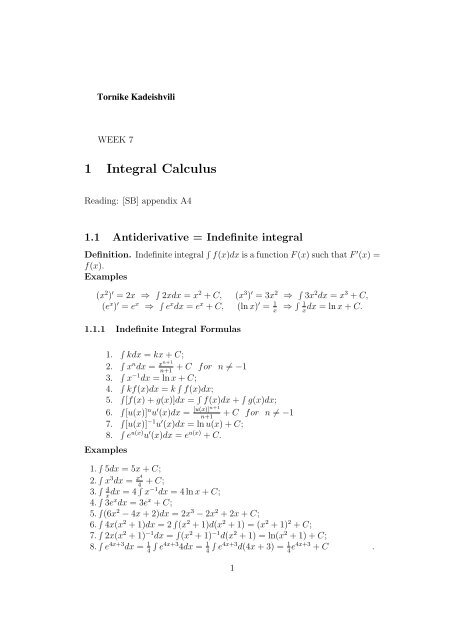
WEEK 7
1 Integral Calculus
Reading: [SB] appendix A4
1.1 Antiderivative = Indefinite integral
Definition. Indefinite integral ∫ f(x)dx is a function F (x) such that F ′ (x) =
f(x).
Examples
(x 2 ) ′ = 2x ⇒ ∫ 2xdx = x 2 + C, (x 3 ) ′ = 3x 2 ⇒ ∫ 3x 2 dx = x 3 + C,
(e x ) ′ = e x ⇒ ∫ e x dx = e x + C, (ln x) ′ = 1 ⇒ ∫ 1dx = ln x + C.
x x
1.1.1 Indefinite Integral Formulas
1.
2.
3.
4.
5.
6.
7.
8.
Examples
∫ kdx = kx + C;
∫ x n dx = xn+1 + C for n ≠ −1
∫ n+1
x −1 dx = ln x + C;
∫ ∫
∫ kf(x)dx = k f(x)dx;
∫ ∫ [f(x) + g(x)]dx = f(x)dx + g(x)dx;
∫ [u(x)] n u ′ (x)dx = [u(x)]n+1 + C for n ≠ −1
∫ n+1
[u(x)] −1 u ′ (x)dx = ln u(x) + C;
∫ e u(x) u ′ (x)dx = e u(x) + C.
1. ∫ 5dx = 5x + C;
2. ∫ x 3 dx = x4 + C; 4
3. ∫ 4
dx = 4 ∫ x −1 dx = 4 ln x + C;
x
4. ∫ 3e x dx = 3e x + C;
5. ∫ (6x 2 − 4x + 2)dx = 2x 3 − 2x 2 + 2x + C;
6. ∫ 4x(x 2 + 1)dx = 2 ∫ (x 2 + 1)d(x 2 + 1) = (x 2 + 1) 2 + C;
7. ∫ 2x(x 2 + 1) −1 dx = ∫ (x 2 + 1) −1 d(x 2 + 1) = ln(x 2 + 1) + C;
8. ∫ e 4x+3 dx = 1 ∫
4 e 4x+3 4dx = 1 ∫
4 e 4x+3 d(4x + 3) = 1 4 e4x+3 + C .
1

Exercises
1.
2.
3.
4.
5.
6.
7.
8.
9.
∫ (2x + 3) 10 dx.
∫ (2x + 3) −1 dx.
∫ (2x + 3) −3 dx.
∫ x(2x 2 + 3) −1 dx.
∫ x 2 (2x 3 + 3) 5 dx.
∫ e 3x dx.
∫ e x (3e x + 1) 7 dx.
∫ x
dx.
3x 2 +1
∫ x 2
dx.
1−3x 3
Find f(x) if
10. f ′ (x) = 2x − 3, and f(0) = 5.
11. f ′ (x) = 2x −2 + 3x −1 and f(1) = 0.
12. Marginal cost function is given by C ′ (x) = 3x 2 − 24x + 53, and the fixed
cost at 0 output are $ 30,000. What is the cost for manufacturing of 4,000
items?
13. The weekly marginal revenue from the sale of x pairs of shoes is given
by R ′ (x) = 40 − 0.02x + 200 . Besides R(0) = 0. Find the revenue function.
x+1
Find the revenue from the sale of 1,000 shoes.
14. The weekly marginal cost of producing x pairs of shoes is C ′ (x) =
12 + 500 , and the weekly fixed costs are $ 2,000. Find the cost function.
x+1
What is the average cost per one pair of shoes if 1,000 pair of shoes are
produced?
1.1.2 Integration by Parts
By product rule
Integrating both sides we obtain
[u(x) · v(x)] ′ = u ′ (x) · v(x) + u(x) · v ′ (x).
∫ [u(x) · v(x)] ′ dx = ∫ u ′ (x) · v(x)dt + ∫ u(x) · v ′ (x)dx,
u(x) · v(x) = ∫ u ′ (x) · v(x)dt + ∫ u(x) · v ′ (x)dx,
let us rewrite this as
∫
∫
u(x) · v ′ (x)dx = u(x) · v(x) −
u ′ (x) · v(x)dx.
Equivalently
∫
∫
u(x) · dv(x) = u(x) · v(x) −
v(x)du(x).
2

Examples
1. Calculate ∫ xe x dx. Let u(x) = x, dv(x) = e x dx, then du(x) = dx and
v(x) = e x thus
∫ xe x dx = ∫ u(x)dv(x) = u(x)v(x) − ∫ v(x)du(x) =
xe x − ∫ e x dx = xe x − e x + C.
2. Calculate ∫ ln xdx. Let u(x) = ln x, dv(x) = dx, then du(x) = 1 dx and
x
v(x) = x thus
∫ ln xdx =
∫ u(x)dv(x) = u(x)v(x) −
∫ v(x)du(x) =
(ln x) · x − ∫ xd(ln x) =
x ln x − ∫ x · 1
x dx = x ln x − ∫ dx = x ln x − x + C.
3. Calculate ∫ x √ x + 1dx. Let u(x) = x, dv(x) = (x + 1) 1 2 dx, then du(x) =
dx and v(x) = ∫ dv(x) = ∫ (x + 1) 1 2 dx = 2(x + 1) 3 2 thus
3
∫ √ ∫ ∫ x x + 1dx = u(x)dv(x) = u(x)v(x) − v(x)du(x) =
x · 2(x
+ 1) 3 2 − ∫ 2
(x + 1) 3 2 dx =
3 3
2
x(x + 1) 3 2 − 2 · (x+1) 3 2 +1
3 3 3 = 2x(x + 1) 3
2 +1 2 − 4 (x + 1) 5 2 + C.
3 15
Exercises
1. Calculate ∫ x ln xdx. Try 4 ways to solve this problem, which way works?
Way 1. Let u(x) = 1,
dv(x) = x ln xdx.
Way 2. Let u(x) = x ln x,
Way 3. Let u(x) = ln x,
dv(x) = dx.
dv(x) = xdx.
Way 4. Let u(x) = x,
dv(x) = ln xdx.
2. Calculate ∫ x 3 · e x dx.
1.2 Definite Integral
The definite integral ∫ b
a f(x)dx is defined as follows. Take any natural number
N and divide the interval [a, b] into N equal subintervals, for this let ∆ = b−a
N
and let’s consider the points
x 0 = a, x 1 = x 0 + ∆, x 2 = x 1 + ∆, ... , x N = x N−1 + ∆ = b,
3

these points divide [a, b] into N intervals
[a = x 0 , x 1 ], [x 1 , x 2 ], ... , [x k , x k+1 ], ... , [x N−1 , x N = b]
each of length ∆.
Now consider the Riemann sum
N∑
f(x 0 )·(x 1 −x 0 )+f(x 1 )·(x 2 −x 1 )+ ... +f(x N−1 )·(x N −x N−1 ) = f(x i−1 )·∆.
i=1
This sum approximates the area under the graph of f(x) from a to b:
Definition. The definite integral ∫ b
a f(x)dx is defined as the limit
N∑
lim f(x i−1 ) · ∆.
N→∞
i=1
Remark. Actually in the general definition of definite integral partitions
of [a, b] not necessarily into equal intervals [x k−1 , x k ] are used, and in the
limit process it is assumed that the length of largest subinterval goes to zero.
Besides, as f(x k ) can be taken not necessarily the left end but any point of
the k-th subinterval [x k−1 , x k ].
1.2.1 The Fundamental Theorem of Calculus
As we see the definitions of indefinite and definite integrals are totally different.
This theorem connects these two notions: suppose F ′ (x) = f(x), i.e.
∫ f(x)dx = F (x) + C, then
∫ b
a
f(x)dx = F (b) − F (a) = F (x)| b a.
Example. Calculate ∫ e
1 ln xdx. 4

Solution. We have already calculated the indefinite integral
∫
ln xdx = x ln x − x + C.
Then ∫ e
1 ln xdx = (x ln x − x + C)|e 1 =
(e · ln e − e + C) − (1 · ln 1 − 1 + C) =
(e − e + C) − (1 · 0 − 1 + C) = 1.
1.3 Applications
1.3.1 Average Value
Let f be a continuous function over a closed interval [a, b]. Its average value
over [a, b] is
y av = 1 ∫ b
f(x)dx.
b − a a
Geometrical meaning: multiply both sides by b − a
(b − a) · y av =
∫ b
a
f(x)dx.
So the average value y av is the height of the rectangle of length b − a whose
area is the same as the area under the graph of f(x) over the interval [a, b],
which equals to ∫ b
a f(x)dx.
Example. Find the average value of f(x) = x 3 over the interval [−1, 1].
Is it strange?
y av =
∫
1 1
x 3 dx = 1 1 − (−1) −1 2 · x4
4 |1 −1 = 1 2 (1 4 − 1 4 ) = 0.
5

1.3.2 Consumer’s Surplus
Consider the inverse demand function p = D(q) (p is the price at the demand
q). We know that this is a decreasing function.
Take any demand q ∗ , the corresponding price is p ∗ = D(q ∗ ). If we purchase
q ∗ units immediately for the price p ∗ = D(q ∗ ), then our expenditure
will be q ∗ · D(q ∗ ).
On the other hand the total willingness to pay for q ∗ units of commodity
is the area under the graph of inverse demand function p = D(q) on the
interval [0, q ∗ ], so it is ∫ q ∗
0 f(q)dq.
The consumer’s surplus is defined as
∫ q ∗
0
D(q)dq − q ∗ · D(q ∗ ).
Example. Let the price of a book depending on number of books purchased
is given by p = 10 − q, this means that the price of the first book is $9; of the
second is $8; of the third book is $7, etc. Let us analyze what does it mean.
Consider three strategies of selling books.
1. Trivial: each book costs 9, so if you buy two books, you pay 9+9=18;
if you buy three books you pay 9+9+9=27, etc.
2. Weak discount: if you buy one book you pay 9; if you buy two books
you pay 9 for the first book and 8 for the second, so 9+8=17 for both; if you
buy three books you pay 9 for the first, 8 for the second, 7 for the third, so
you pay 9+8+7=25 for all three, etc.
3. Strong discount: if you buy one book you pay 9; if you buy two
books you pay 8 for each, so you pay 8+8=16 for both; if you buy three
books you pay 7 for each, so you pay 7+7+7=21 for all three, etc.
The consumer’s surplus is the difference between the second and the third
methods, that is:
6

If q = 1, the surplus is 9-9=0.
If q = 2, the surplus is 17-16=1.
If q = 3, the surplus is 25-21=4.
Generally, if q = q 0 , the surplus is
∫ q0
0 (10 − q)dq − q 0 · (10 − q 0 ) = (10q − q2 2 )|q 0
0 − 10q 0 + q 2 0 =
10q 0 − q2 0
2
− 10q 0 + q 2 0 = q2 0
2
.
Why this result differs from above for q 0 = 1, 2, 3?
1.3.3 Producer’s Surplus
Let p = S(q) be the supply function for a commodity, it is an increasing
function. The producer’s surplus at q = q ∗ is defined as
q ∗ · S(q ∗ ) −
∫ q ∗
0
S(q)dq.
Example. Let D(q) = (q − 5) 2 and S(q) = q 2 + q + 3, find
(a) The equilibrium point.
(b) The consumer’s surplus at the equilibrium point.
(c) The producer’s’s surplus at the equilibrium point.
7

Solution.
(a) S(q) = D(q), (q − 5) 2 = q 2 + q + 3, q ∗ = 2, p ∗ = D(2) = S(2) = 9.
(b)
∫ 2
0
D(q)dq − q ∗ · D(q ∗ ) =
∫ 2
0
(q − 5) 2 dq − 2 · 9 =
(q − 5)3
| 2 0 − 18 = 44 3
3 .
(c) q ∗·S(q ∫ 2
∫ 2
∗ )− S(q)dq = 2·9− (q 2 +q+3)dq = 18−( (q3
0
0
3 + q2
2 +q)|2 0 = 22 3 .
8

Exercises
A4.1-A4.5 from [SB], pp. 983.
1. Find the consumer’s surplus at a price level $150 if the price-demand
equation is D(x) = 400 − 0.05x.
2. Find the producer’s surplus at a price level $67 if the price-supply
equation is S(x) = 10 + 0.1x + 0.0003x 2 .
3. Suppose the price-demand function is D(x) = 50 − 0.1x and the pricesupply
function is S(x) = 11 + 0.05x. Find:
(a) The equilibrium price level.
(b) Consumer’s surplus at equilibrium.
(c) Producer’s surplus at equilibrium.
9