Earned Schedule Analysis, A Better Set of Schedule Metrics
Earned Schedule Analysis, A Better Set of Schedule Metrics
Earned Schedule Analysis, A Better Set of Schedule Metrics

You also want an ePaper? Increase the reach of your titles
YUMPU automatically turns print PDFs into web optimized ePapers that Google loves.
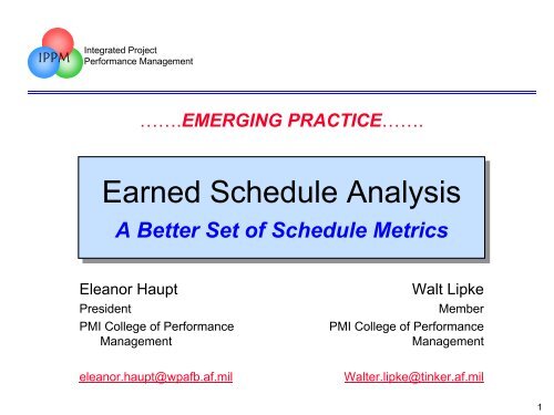
IPPM<br />
Integrated Project<br />
Performance Management<br />
…….EMERGING PRACTICE…….<br />
<strong>Earned</strong> <strong>Schedule</strong> <strong>Analysis</strong><br />
A <strong>Better</strong> <strong>Set</strong> <strong>of</strong> <strong>Schedule</strong> <strong>Metrics</strong><br />
Eleanor Haupt<br />
President<br />
PMI College <strong>of</strong> Performance<br />
Management<br />
Walt Lipke<br />
Member<br />
PMI College <strong>of</strong> Performance<br />
Management<br />
eleanor.haupt@wpafb.af.mil<br />
Walter.lipke@tinker.af.mil<br />
1
IPPM<br />
***CAUTION***<br />
…….EMERGING PRACTICE…….<br />
Use with caution until validated by by research.<br />
Do not substitute for for analysis <strong>of</strong> <strong>of</strong> integrated master<br />
schedule.<br />
2
IPPM<br />
Overview<br />
• How earned schedule was developed<br />
• Basic concepts <strong>of</strong> earned schedule<br />
• Management uses<br />
• Benefits<br />
• Way ahead<br />
3
IPPM<br />
How <strong>Earned</strong> <strong>Schedule</strong> was<br />
Developed<br />
4
IPPM<br />
Traditional Definition<br />
<strong>Schedule</strong> Performance Index<br />
NOTIONAL DATA<br />
1.2<br />
1.1<br />
1.0<br />
.9<br />
TIME<br />
SPI<br />
.8<br />
SPI = Work Performed = BCWP<br />
Work <strong>Schedule</strong>d BCWS<br />
calculated from budgeted cost<br />
5
IPPM<br />
SPI at the End <strong>of</strong> the Project<br />
NOTIONAL DATA<br />
1.2<br />
1.1<br />
Project status:<br />
Project finished 3 months late<br />
Final SPI = 1.00<br />
Final SV$ = 0<br />
There’s got to<br />
be a better<br />
metric!<br />
3 months<br />
1.0<br />
.9<br />
TIME<br />
SPI<br />
.8<br />
Original<br />
Project<br />
Finish<br />
Actual<br />
Project<br />
Finish<br />
6
IPPM<br />
The Problem with Traditional EVM<br />
<strong>Schedule</strong> <strong>Metrics</strong><br />
• Traditional schedule EVM metrics are good at beginning <strong>of</strong><br />
project<br />
– Show schedule performance trends<br />
• But the metrics don’t reflect real schedule performance at end<br />
– Eventually, all “budget” will be earned as the work is completed,<br />
no matter how late you finish<br />
• SPI improves and ends up at 1.00 at end <strong>of</strong> project<br />
• SV improves and ends up at $0 variance<br />
• Traditional schedule metrics lose their predictive ability over the last<br />
third <strong>of</strong> project<br />
• Impacts schedule predictions, EAC predictions<br />
• Project managers don’t understand schedule<br />
performance in terms <strong>of</strong> budget<br />
– Like most <strong>of</strong> us!<br />
7
IPPM<br />
The Beginning <strong>of</strong> <strong>Earned</strong> <strong>Schedule</strong><br />
• Seeking a statistical application to s<strong>of</strong>tware management<br />
– A growing trend in the s<strong>of</strong>tware industry<br />
– Had become a requirement for SEI CMM Level 4<br />
• Chose CPI & SPI instead <strong>of</strong> a quality metric (e.g., defects / LOC)<br />
– More meaningful application …the system vice a component<br />
• Vision …the application could provide …<br />
– Greater process understanding<br />
– Improved planning …a probabilistic treatment <strong>of</strong> Risk<br />
– <strong>Better</strong> outcome prediction …the probability <strong>of</strong> success<br />
– Long term process improvement indicators<br />
• Inherent failure <strong>of</strong> SPI …statistics must have reliable numbers<br />
– Experiment …schedule accomplishment <strong>of</strong> PMB resolves EVM flaw<br />
• Published result in Spring 2003 The Measurable News<br />
– Kym Henderson phoned from Australia … “It works!!”<br />
– IPMC 2003 & CPM 2004 …Eleanor has been a strong advocate<br />
8
IPPM<br />
References<br />
• Lipke, Walt, <strong>Schedule</strong> is Different, Measurable News, College <strong>of</strong><br />
Performance Management, March 2003 (reprinted Summer 2003)<br />
• Henderson, Kym, <strong>Earned</strong> <strong>Schedule</strong>: A Breakthrough Extension to<br />
<strong>Earned</strong> Value Theory? A Retrospective <strong>Analysis</strong> <strong>of</strong> Real Project Data,<br />
Measurable News, College <strong>of</strong> Performance Management, Summer<br />
2003<br />
• Henderson, Kym, Further Developments in <strong>Earned</strong> <strong>Schedule</strong>,<br />
Measurable News, College <strong>of</strong> Performance Management, Spring 2004<br />
9
IPPM<br />
Basic Concepts <strong>of</strong> <strong>Earned</strong><br />
<strong>Schedule</strong><br />
10
IPPM<br />
<strong>Earned</strong> <strong>Schedule</strong> Concepts<br />
• Analogous to <strong>Earned</strong> Value<br />
– Based on time-phased earned value data (BCWS, BCWP)<br />
• However, schedule performance is determined with time<br />
based metrics, not cost<br />
– Key concept: how much schedule did I earn on the BCWS curve?<br />
– Resulting metrics and variances are expressed in time units<br />
– Works for both conditions (ahead or behind schedule)<br />
• Bridge between traditional EVM and integrated scheduling<br />
– Correlation requires certain data from integrated master schedule<br />
(IMS)<br />
– Does not replace need to maintain and analyze IMS<br />
11
IPPM<br />
What Data do I Need?<br />
• EVM data<br />
– BCWP cum to date<br />
– BCWS cum to date (from beginning to time now)<br />
• Integrated Master <strong>Schedule</strong> data<br />
– Start date<br />
– Planned completion date (baseline)<br />
– Planned duration (without total float)<br />
– Total schedule float (days)<br />
– Estimated completion date<br />
– Optional:<br />
• Unconstrained completion date<br />
Hey, I’ve<br />
got that<br />
data!<br />
12
IPPM<br />
Determining <strong>Earned</strong> <strong>Schedule</strong><br />
How Much <strong>Schedule</strong> Did I Earn?<br />
• <strong>Earned</strong> <strong>Schedule</strong> = cumulative earned value in time units<br />
as established by the value <strong>of</strong> cumulative BCWP on the BCWS<br />
curve<br />
– Partial units <strong>of</strong> time are calculated<br />
• Can be calculated graphically or with tabular data<br />
$<br />
BCWS<br />
EARNED<br />
SCHEDULE<br />
=<br />
~6.1 months<br />
BCWP<br />
•• Actual Actual time time is is 9 months<br />
•• The The earned earned schedule is is<br />
6.1 6.1 months<br />
6<br />
9<br />
Actual<br />
Time<br />
Months<br />
13
IPPM<br />
<strong>Earned</strong> <strong>Schedule</strong> <strong>Metrics</strong><br />
SV(t) = <strong>Schedule</strong> Variance (time)<br />
= <strong>Earned</strong> <strong>Schedule</strong> – Actual Time<br />
= 6.1 months – 9 months<br />
= -2.9 months<br />
I should have<br />
earned 9 months,<br />
but have only<br />
earned 6.1 months<br />
SPI(t) = <strong>Schedule</strong> Performance Index (time)<br />
= <strong>Earned</strong> <strong>Schedule</strong> = 6.1 = .68<br />
Actual Time 9<br />
14
IPPM<br />
SV($) versus SV(t)<br />
BCWS<br />
$<br />
SV($)<br />
<strong>Earned</strong> <strong>Schedule</strong> (ES)<br />
BCWP<br />
SV(t)<br />
•• <strong>Earned</strong> schedule metrics relate relate<br />
work work performed to to actual actual time, time,<br />
not not work work scheduled<br />
•• Retain Retain utility utility over over time time<br />
•• never never return return to to 0 or or 1.00 1.00<br />
Actual Actual Time Time<br />
15
IPPM<br />
SPI(t) at the End <strong>of</strong> the Project<br />
1.2<br />
1.1<br />
Project Project status: status:<br />
Project Project finished finished 3 months months late late<br />
Final Final SPI(t) SPI(t) = .88 .88<br />
Final Final SV(t) SV(t) = -3 -3 months<br />
3 months<br />
1.0<br />
.9<br />
.8<br />
TIME<br />
SPI(t)<br />
Original<br />
Project<br />
Finish<br />
Actual<br />
Project<br />
Finish<br />
16
IPPM<br />
Management Uses<br />
17
IPPM<br />
How to Gain the Attention <strong>of</strong> the<br />
Project Manager<br />
• Evaluate and show trends against baseline schedule<br />
• Predict a range <strong>of</strong> durations<br />
• Evaluate realism <strong>of</strong> contractor’s schedule estimate<br />
• Show a range <strong>of</strong> completion dates<br />
• Compare ES trends to integrated master schedule<br />
18
<strong>Earned</strong> <strong>Schedule</strong> vs. Planned Duration<br />
25<br />
NOTIONAL DATA<br />
PCD<br />
20<br />
Duration (Months)<br />
15<br />
10<br />
5<br />
<strong>Analysis</strong><br />
The baselined duration is 23 months,<br />
which means that the project should<br />
finish in Dec 04. However, schedule<br />
performance for the past six months<br />
has degraded. We are not making<br />
schedule and the trend is growing<br />
worse.<br />
Planned Duration (PD) (months)<br />
<strong>Earned</strong> <strong>Schedule</strong> (ES) (months)<br />
0<br />
Feb-<br />
03<br />
Mar-<br />
03<br />
Apr-<br />
03<br />
May-<br />
03<br />
Jun-<br />
03<br />
Jul-<br />
03<br />
Aug-<br />
03<br />
Sep-<br />
03<br />
Oct-<br />
03<br />
Nov-<br />
03<br />
Dec-<br />
03<br />
Jan-<br />
04<br />
Feb-<br />
04<br />
Mar-<br />
04<br />
Apr-<br />
04<br />
May-<br />
04<br />
Jun-<br />
04<br />
Jul-<br />
04<br />
Aug-<br />
04<br />
Sep-<br />
04<br />
Oct-<br />
04<br />
Nov-<br />
04<br />
Dec-<br />
04<br />
Actual Time<br />
NOTE: the dashed line is a straight line, as it represents that we should be earning one month <strong>of</strong><br />
schedule for each elapsed month. This is not a BCWS curve.
IPPM<br />
Predicting Durations?<br />
• EVM<br />
– CPI has proven to be stable metric<br />
• Used to predict estimated final costs<br />
– SPI($) rarely used to predict duration<br />
• <strong>Earned</strong> <strong>Schedule</strong><br />
– Early work by Kym Henderson indicates stability <strong>of</strong> SPI(t)<br />
– How can SPI(t) be used to predict duration?<br />
20
IPPM<br />
Predicting the Duration<br />
IEAC(t) = Independent Estimate at Completion (Time)<br />
= Planned Duration = 23 months<br />
SPI(t) .68<br />
= 33.8 months<br />
Parallels EAC formula based on CPI<br />
Assumes schedule performance will remain at same efficiency<br />
Use Use this this as as crosscheck against baseline<br />
or or revised estimate <strong>of</strong> <strong>of</strong> schedule<br />
21
RANGE OF DURATION ESTIMATES<br />
36.00<br />
34.00<br />
MONTHS<br />
32.00<br />
30.00<br />
28.00<br />
26.00<br />
PD<br />
EAC(t) (contractor)<br />
Unconstrained<br />
IEAC(t) (customer)<br />
24.00<br />
22.00<br />
20.00<br />
Feb-03 Mar-03 Apr-03 May-03 Jun-03 Jul-03 Aug-03 Sep-03 Oct-03 Nov-03<br />
TIME<br />
<strong>Analysis</strong><br />
Even though the contractor has provided an<br />
updated schedule estimate, it appears that it<br />
is unachievable. The independent<br />
calculation by the customer results in an<br />
estimated duration <strong>of</strong> just under 34 months,<br />
compared to the contractor’s estimate <strong>of</strong> 25<br />
months.<br />
Recommend calculation <strong>of</strong> a<br />
range <strong>of</strong> durations
IPPM<br />
Evaluate Realism <strong>of</strong> Contractor’s<br />
<strong>Schedule</strong><br />
Compare Past to Future Efficiency<br />
Past <strong>Schedule</strong> Efficiency = SPI(t)<br />
= <strong>Earned</strong> <strong>Schedule</strong><br />
Actual Time<br />
.68 .68<br />
Future <strong>Schedule</strong> Efficiency = To complete <strong>Schedule</strong><br />
Performance Index (time)<br />
COMPARE<br />
= TSPI<br />
1.06 1.06<br />
= Planned Duration for Work Remaining<br />
Time Estimate to Complete<br />
Future efficiency needed to achieve contractor’s revised estimate <strong>of</strong> duration<br />
23
SPI(t) versus TSPI(t)<br />
1.20<br />
1.00<br />
Future efficiency needed to<br />
achieve estimated schedule<br />
0.80<br />
0.60<br />
actual efficiency achieved to date<br />
0.40<br />
0.20<br />
<strong>Analysis</strong><br />
This shows the past efficiency<br />
versus the efficiency needed to<br />
achieve the contractor’s revised<br />
estimate. There is a large gap that<br />
is worsening, indicating that the<br />
revised estimate is unachievable.<br />
SPI(t)<br />
TSPI<br />
0.00<br />
Feb-03 Mar-03 Apr-03 May-03 Jun-03 Jul-03 Aug-03 Sep-03 Oct-03
COMPLETION DATES<br />
24-Mar-06<br />
14-Dec-05<br />
5-Sep-05<br />
28-May-05<br />
17-Feb-05<br />
9-Nov-04<br />
1-Aug-04<br />
PCD<br />
ECD (contractor)<br />
23-Apr-04<br />
14-Jan-04<br />
<strong>Analysis</strong><br />
These projected completion dates are based<br />
on the estimated durations and are shown<br />
over time. The independent estimate shows<br />
a completion <strong>of</strong> 24 Nov 05, versus the<br />
baselined date <strong>of</strong> 31 Dec 04, a slip <strong>of</strong> 11<br />
months. Contractor’s schedule appears<br />
unachievable.<br />
Feb-03 Mar-03 Apr-03 May-03 Jun-03 Jul-03 Aug-03 Sep-03 Oct-03<br />
TIME<br />
Unconstrained<br />
IECD (customer)
SPI(t) versus Total Float<br />
1.20<br />
0.80<br />
0.70<br />
1.00<br />
0.60<br />
0.80<br />
0.50<br />
SPI(t)<br />
0.60<br />
0.40<br />
0.20<br />
<strong>Analysis</strong><br />
This compares the trend in the<br />
schedule efficiency versus the<br />
amount <strong>of</strong> total float in the schedule.<br />
In this case, schedule efficiency has<br />
been declining and is poor. The red<br />
line shows the change in total float<br />
(in months), indicating that total float<br />
is now negative.<br />
SPI(t)<br />
Total Float (months)<br />
0.40<br />
0.30<br />
0.20<br />
0.10<br />
0.00<br />
-0.10<br />
Total Float (months)<br />
0.00<br />
Feb-03 Mar-03 Apr-03 May-03 Jun-03 Jul-03 Aug-03 Sep-03 Oct-03<br />
-0.20
IPPM<br />
Efficiencies vs. Completion Dates<br />
<strong>Schedule</strong> Performance Index (Time)<br />
1.2<br />
1.1<br />
1.0<br />
.9<br />
.8<br />
<strong>Analysis</strong><br />
This shows the actual efficiency and<br />
schedule trend against the end date<br />
<strong>of</strong> the contract and against the<br />
unconstrained end date. Based on<br />
this efficiency, it is likely that the<br />
project will not make the contract<br />
end date.<br />
Contract <strong>Schedule</strong> Efficiency<br />
(indicates efficiency needed to stay within<br />
contract dates)<br />
SPI(t)<br />
Time<br />
Unconstrained <strong>Schedule</strong> Efficiency<br />
(indicates efficiency needed to stay within<br />
unconstrained schedule dates)<br />
Contract<br />
End Date<br />
Unconstrained<br />
End Date<br />
27
IPPM<br />
Help!<br />
I’m a little overwhelmed…<br />
28
New Terminology Parallels EVM Terminology<br />
Status<br />
<strong>Earned</strong> Value (EV)<br />
Actual Costs (AC)<br />
EVMS<br />
<strong>Earned</strong> <strong>Schedule</strong><br />
<strong>Earned</strong> <strong>Schedule</strong> (ES)<br />
Actual Time (AT)<br />
Future Work<br />
Final Status<br />
SV($)<br />
SPI($)<br />
Budgeted Cost for Work Remaining<br />
(BCWR)<br />
Estimate to Complete (ETC)<br />
Variance at Completion<br />
(VAC)<br />
Estimate at Completion (EAC)<br />
(contractor)<br />
SV(t)<br />
SPI(t)<br />
Planned Duration for Work<br />
Remaining (PDWR)<br />
Estimate to Complete (time)<br />
ETC(t)<br />
Variance at Completion (time)<br />
VAC(t)<br />
Estimate at Completion (time)<br />
EAC(t) (contractor)<br />
Independent EAC<br />
(IEAC)<br />
(customer)<br />
Independent Estimate at<br />
Completion (time)<br />
IEAC(t) (customer)
<strong>Earned</strong> <strong>Schedule</strong> Excel worksheet<br />
Contains logic, formulas, generates charts<br />
Month Feb-03 Mar-03 Apr-03 May-03 Jun-03 Jul-03 Aug-03 Sep-03 Oct-03<br />
BCWScum ($) 782 1,411 1,923 2,510 3,215 4,127 5,122 6,229 7,279<br />
BCWPcum ($) 804 1,423 1,687 1,886 2,304 2,751 3,198 3,801 4,257<br />
Status to Date<br />
Actual Time (AT) (months) 1.00 2.00 3.00 4.00 5.00 6.00 7.00 8.00 9.00<br />
<strong>Earned</strong> <strong>Schedule</strong> (ES) (months) 1.03 2.02 2.54 2.93 3.65 4.34 4.98 5.64 6.13<br />
Planned Duration for Work Remaining<br />
(PDWR) 21.98 20.99 20.47 20.09 19.36 18.67 18.04 17.37 16.88<br />
SV(t) (months) 0.03 0.02 -0.46 -1.07 -1.35 -1.66 -2.02 -2.36 -2.87<br />
SV(t) % 3% 1% -15% -27% -27% -28% -29% -29% -32%<br />
SPI(t) 1.03 1.01 0.85 0.73 0.73 0.72 0.71 0.71 0.68<br />
At Completion<br />
BLUE FONT INDICATES DATA ENTRY CELLS<br />
Project Start 1-Feb-03 1-Feb-03 1-Feb-03 1-Feb-03 1-Feb-03 1-Feb-03 1-Feb-03 1-Feb-03 1-Feb-03<br />
Planned Completion Date (PCD)<br />
31-Dec-04 31-Dec-04 31-Dec-04 31-Dec-04 31-Dec-04 31-Dec-04 31-Dec-04 31-Dec-04 31-Dec-04<br />
Estimated Completion Date (ECD) 31-Dec-04 31-Dec-04 5-Jan-05 5-Jan-05 5-Jan-05 23-Jan-05 28-Feb-05 28-Feb-05 28-Feb-05<br />
Contract Completion Date 22-Jan-05 22-Jan-05 22-Jan-05 22-Jan-05 22-Jan-05 22-Jan-05 22-Jan-05 22-Jan-05 22-Jan-05<br />
Total Float (days) 22 22 21 19 17 12 8 1 -2<br />
Total Float (months) 0.72 0.72 0.69 0.62 0.56 0.39 0.26 0.03 -0.07<br />
Unconstrained Duration (months) 27.00 27.00 27.00 28.00 29.00 32.00 32.00 32.00 32.00<br />
Unconstrained <strong>Schedule</strong> Efficiency (USE) 0.85 0.85 0.85 0.82 0.79 0.72 0.72 0.72 0.72<br />
Unconstrained Completion Date 2-May-05 2-May-05 2-May-05 1-Jun-05 2-Jul-05 1-Oct-05 1-Oct-05 1-Oct-05 1-Oct-05<br />
available upon request<br />
for use or evaluation<br />
NOTIONAL DATA<br />
Planned Duration (PD) (months) 23.01 23.01 23.01 23.01 23.01 23.01 23.01 23.01 23.01<br />
Estimate at Completion (time) EAC(t)<br />
(months) 23.01 23.01 23.18 23.18 23.18 23.77 24.95 24.95 24.95<br />
Estimate to Completion (time) ETC(t)<br />
(months) 22.01 21.01 20.18 19.18 18.18 17.77 17.95 16.95 15.95<br />
Variance at Completion (time) VAC(t)<br />
(months) 0.00 0.00 -0.16 -0.16 -0.16 -0.76 -1.94 -1.94 -1.94<br />
Independent Estimate at Completion (time)<br />
IEAC(t)<br />
AT + PDWR 22.98 22.99 23.47 24.09 24.36 24.67 25.04 25.37 25.88<br />
AT + PDWR + Total Float 23.70 23.71 24.17 24.71 24.92 25.07 25.30 25.40 25.88<br />
PD / SPI(t) 22.24 22.75 27.19 31.44 31.53 31.80 32.38 32.63 33.78<br />
PD / SPI(t) + Total Float 22.96 23.47 27.88 32.07 32.09 32.20 32.64 32.66 33.78<br />
(PD + TF) / SPI(t) 22.93 23.46 28.01 32.30 32.30 32.35 32.75 32.68 33.78<br />
AT + (PDWR / USE) 26.79 26.63 27.02 28.44 29.40 31.96 32.08 32.15 32.48<br />
Independent Estimated Completion Date<br />
(using SPI(t)) 8-Dec-04 23-Dec-04 8-May-05 14-Sep-05 17-Sep-05 25-Sep-05 12-Oct-05 20-Oct-05 24-Nov-05<br />
Comparison <strong>of</strong> Indices<br />
SPI(t) 1.03 1.01 0.85 0.73 0.73 0.72 0.71 0.71 0.68<br />
TSPI 1.00 1.00 1.01 1.05 1.07 1.05 1.00 1.02 1.06<br />
Projected Final SPI(t) 1.00 1.00 0.99 0.99 0.99 0.97 0.92 0.92 0.92<br />
Contract Efficiencies<br />
Contract Duration 23.74 23.74 23.74 23.74 23.74 23.74 23.74 23.74 23.74<br />
Contract <strong>Schedule</strong> Efficiency 0.97 0.97 0.97 0.97 0.97 0.97 0.97 0.97 0.97<br />
Unconstrained <strong>Schedule</strong> Efficiency 0.85 0.85 0.85 0.82 0.79 0.72 0.72 0.72 0.72<br />
SPI(t) 1.03 1.01 0.85 0.73 0.73 0.72 0.71 0.71 0.68<br />
EARNED EARNED SCHEDULE<br />
SCHEDULE<br />
= (HLOOKUP(J5,$B$3:$X$5,2))+(J5-<br />
(HLOOKUP(J5,$B$3:$X$5,1)))/((HLOOKUP(<br />
((HLOOKUP(J5,$B$3:$X$5,2))+1),$B$7:$X$<br />
8,2)-(HLOOKUP(J5,$B$3:$X$5,1))))<br />
Eleanor<br />
I’m out<br />
<strong>of</strong> brain<br />
cells
IPPM<br />
Benefits<br />
31
IPPM<br />
Benefits <strong>of</strong> <strong>Earned</strong> <strong>Schedule</strong><br />
• Makes common sense!<br />
• Easier concept to grasp<br />
– <strong>Schedule</strong> variance metrics in terms <strong>of</strong> time rather than $<br />
• More stable metric<br />
– Retains trend until end <strong>of</strong> project<br />
– Retains predictive utility<br />
• Use to predict duration<br />
• Can be used to improve EAC predictions<br />
– Check <strong>of</strong> contractor’s schedule realism<br />
• Bridge between EVM and the integrated master<br />
schedule<br />
32
IPPM<br />
The Way Ahead<br />
33
IPPM<br />
Research Topics<br />
• Determine if SPI(t) is a valid predictor <strong>of</strong> final<br />
duration (ongoing graduate thesis)<br />
• Validate use <strong>of</strong> SPI(t) in EAC formulas<br />
• Determine if earned schedule metrics are better at<br />
portraying schedule performance than traditional<br />
EVM metrics<br />
– Demonstrated on pilot projects<br />
– Need demonstration on broader scope <strong>of</strong> projects<br />
• Compare predicted IEAC(t) durations against<br />
predicted critical path<br />
34
IPPM<br />
Impact to EAC Formulas<br />
• Performance based EAC formulas<br />
– Two formulas rely on SPI($)<br />
• But, predictive ability is lost during late stage <strong>of</strong> project<br />
– Need to determine applicability <strong>of</strong> using SPI(t) in EAC formulas<br />
• Weighted performance factor: .5*CPI + .5*SPI(t)<br />
• Composite performance factor: CPI*SPI(t)<br />
– Analysts should use with caution until research confirms utility<br />
• “Burn rate” analysis<br />
– Use average burn rates (actual cost per month) against<br />
estimates <strong>of</strong> duration<br />
– Should improve EAC projections<br />
35
IPPM<br />
Conclusions<br />
• <strong>Earned</strong> <strong>Schedule</strong><br />
– a powerful new dimension to Integrated Project<br />
Performance Management (IPPM)<br />
– should replace traditional EVM schedule metrics<br />
– a breakthrough in theory and application<br />
the first scheduling system<br />
36