1 Matrix Algebra
1 Matrix Algebra
1 Matrix Algebra

You also want an ePaper? Increase the reach of your titles
YUMPU automatically turns print PDFs into web optimized ePapers that Google loves.
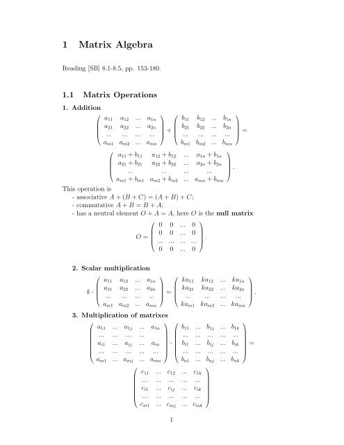
1 <strong>Matrix</strong> <strong>Algebra</strong><br />
Reading [SB] 8.1-8.5, pp. 153-180.<br />
1.1 <strong>Matrix</strong> Operations<br />
1. Addition<br />
⎛<br />
⎜<br />
⎝<br />
⎞ ⎛<br />
a 11 a 12 ... a 1n<br />
a 21 a 22 ... a 2n<br />
⎟<br />
... ... ... ... ⎠ + ⎜<br />
⎝<br />
a m1 a m2 ... a mn<br />
⎛<br />
⎜<br />
⎝<br />
⎞<br />
b 11 b 12 ... b 1n<br />
b 21 b 22 ... b 2n<br />
⎟<br />
... ... ... ... ⎠ =<br />
b m1 b m2 ... b mn<br />
⎞<br />
a 11 + b 11 a 12 + b 12 ... a 1n + b 1n<br />
a 21 + b 21 a 22 + b 22 ... a 2n + b 2n<br />
⎟<br />
... ... ... ... ⎠ .<br />
a m1 + b m1 a m2 + b m2 ... a mn + b mn<br />
This operation is<br />
- associative A + (B + C) = (A + B) + C;<br />
- commutative A + B = B + A;<br />
- has a neutral element O + A = A, here O is the null matrix<br />
⎛<br />
O = ⎜<br />
⎝<br />
0 0 ... 0<br />
0 0 ... 0<br />
... ... ... ...<br />
0 0 ... 0<br />
⎞<br />
⎟<br />
⎠ .<br />
2. Scalar multiplication<br />
⎛<br />
⎞ ⎛<br />
a 11 a 12 ... a 1n<br />
a<br />
k · 21 a 22 ... a 2n<br />
⎜<br />
⎟<br />
⎝ ... ... ... ... ⎠ = ⎜<br />
⎝<br />
a m1 a m2 ... a mn<br />
⎞<br />
ka 11 ka 12 ... ka 1n<br />
ka 21 ka 22 ... ka 2n<br />
⎟<br />
... ... ... ... ⎠ .<br />
ka m1 ka m2 ... ka mn<br />
3. Multiplication of matrixes<br />
⎛<br />
⎞ ⎛<br />
⎞<br />
a 11 ... a 1j ... a 1n b 11 ... b 1j ... b 1k<br />
... ... ... ...<br />
... ... ... ... ...<br />
a i1 ... a ij ... a in<br />
·<br />
b i1 ... b ij ... b ik<br />
=<br />
⎜<br />
⎟ ⎜<br />
⎟<br />
⎝ ... ... ... ... ... ⎠ ⎝ ... ... ... ... ... ⎠<br />
a m1 ... a mj ... a mn b n1 ... b nj ... b nk<br />
⎛<br />
⎜<br />
⎝<br />
⎞<br />
c 11 ... c 12 ... c 1k<br />
... ... ... ... ...<br />
c i1 ... c ij ... c ik<br />
⎟<br />
... ... ... ... ... ⎠<br />
c m1 ... c mj ... c mk<br />
1
where<br />
n∑<br />
c ij = a i1 b 1j + ... + a ik b kj + ... + a in b nj = a ik b kj<br />
k=1<br />
1.2 Transpose of a matrix<br />
Transpose of a m × n matrix A is the n × m matrix A T whose i-th column<br />
is is the i-th row of A.<br />
⎛ ⎞<br />
( )<br />
1 4<br />
1 2 3<br />
For example the transpose for A =<br />
is A<br />
4 5 6<br />
T ⎜ ⎟<br />
= ⎝ 2 5 ⎠.<br />
3 6<br />
Properties of transposes<br />
1. (A T ) T = A;<br />
2. (A + B) T = A T + B T ;<br />
3. (A · B) T = B T · A T .<br />
1.3 Multiplication matrix × column vector<br />
⎛<br />
⎜<br />
⎝<br />
⎞<br />
a 11 a 12 ... a 1n<br />
a 21 a 22 ... a 2n<br />
⎟<br />
... ... ... ... ⎠ ·<br />
a m1 a m2 ... a mn<br />
⎛<br />
⎜<br />
⎝<br />
thus a system of linear equations<br />
⎧<br />
⎪⎨<br />
⎪⎩<br />
can be written in matrix form as<br />
or<br />
⎛<br />
⎜<br />
⎝<br />
⎞<br />
x 1<br />
x 2<br />
⎟<br />
...<br />
x n<br />
⎛<br />
⎠ = ⎜<br />
⎝<br />
a 11 x 1 + a 12 x 2 + ... + a 1n x n = c 1<br />
a 21 x 1 + a 22 x 2 + ... + a 2n x n = c 2<br />
.......................................<br />
a m1 x 1 + a m2 x 2 + ... + a mn x n = c m .<br />
⎞<br />
a 11 a 12 ... a 1n<br />
a 21 a 22 ... a 2n<br />
⎟<br />
... ... ... ... ⎠ ·<br />
a m1 a m2 ... a mn<br />
⎞<br />
a 11 x 1 + a 12 x 2 + ... + a 1n x n<br />
a 21 x 1 + a 22 x 2 + ... + a 2n x n<br />
⎟<br />
....................................... ⎠<br />
a m1 x 1 + a m2 x 2 + ... + a mn x n<br />
⎛<br />
⎜<br />
⎝<br />
A · x = c.<br />
1.4 Special Kinds of Matrices<br />
⎞<br />
x 1<br />
x 2<br />
⎟<br />
...<br />
x n<br />
⎛<br />
⎠ = ⎜<br />
⎝<br />
⎞<br />
c 1<br />
c 2<br />
⎟<br />
... ⎠<br />
c n<br />
Bellow k denotes the number of rows and n denotes the number of columns.<br />
Square matrix. k = n.<br />
Column matrix. n = 1.<br />
2
Row matrix. k = 1.<br />
Diagonal matrix. k = n and a ij = 0 for i ≠ j.<br />
What can you say about the product of two diagonal matrices?<br />
Upper-triangular matrix. k = n and a ij = 0 for i > j.<br />
What can you say about the product of two upper-triangular matrices?<br />
Lower-triangular matrix. k = n and a ij = 0 for i < j.<br />
What can you say about the product of two lower-triangular matrices?<br />
Symmetric matrix. a ij = a ji , equivalently A T = A.<br />
Is a symmetric matrix necessarily square matrix?<br />
What can you say about the product of two symmetric matrices?<br />
Idempotent matrix. A · A = A.<br />
Is an idempotent matrix necessarily square matrix?<br />
What can you say about the determinant of an idempotent matrix?<br />
What can you say about a nonsingular idempotent matrix?<br />
Orthogonal matrix. A −1 = A T .<br />
What can you say about the determinant of an orthogonal matrix?<br />
What can you say about the inverse of an orthogonal matrix?<br />
What can you say about the transpose of an orthogonal matrix?<br />
What can you say about the product of two orthogonal matrices?<br />
What can you say about the sum of two orthogonal matrices?<br />
Involutory matrix. A · A = I.<br />
Is an involutory matrix necessarily square matrix?<br />
What can you say about the determinant of an involutory matrix?<br />
What can you say about the inverse of an involutory matrix?<br />
What can you say about a singular involutory matrix?<br />
What can you say about the transpose of an involutory matrix?<br />
What can you say about the symmetric involutory matrix?<br />
Nilpotent matrix. k = n and A m = 0 for some positive integer m.<br />
Permutation matrix. k = n and each row and each column contains<br />
exactly one 1 and all other entries are 0.<br />
Non singular matrix. k = n is an invertible = nonzero determinant =<br />
maximal rank (see bellow).<br />
3
2 <strong>Algebra</strong> of Square Matrices<br />
The sum, difference, product of square n × n matrices is n × n again, besides<br />
the n × n identity matrix I is true multiplicative identity<br />
I · A = A · I = A.<br />
So the set of all n × n matrices M n carries algebraic structure similar to that<br />
of real numbers R. But there are some differences:<br />
1. Multiplication in M n is not commutative: generally A · B ≠ B · A.<br />
2. M n has zero divisors: there exist nonzero matrices A, B ∈ M n such<br />
that A · B = O.<br />
3. Not all nonzero matrices have inverse.<br />
2.1 Inverse <strong>Matrix</strong><br />
Definition. A matrix A ∈ M n is called invertible there exists its inverse, a<br />
matrix A −1 such that<br />
A · A −1 = A −1 · A = I.<br />
Theorem. An n × n matrix A can have at most one inverse.<br />
Proof. Suppose A −1 and Ā−1 are two inverses for A. Then from one hand<br />
side<br />
A −1 · A · Ā−1 = A −1 · (A · Ā−1 ) = A −1 · I = A −1 ,<br />
and from another hand side<br />
A −1 · A · Ā−1 = (A −1 · A) · Ā−1 = I · Ā−1 = Ā−1<br />
thus A −1 = A −1 · A · Ā−1 = Ā−1 .<br />
2.1.1 Some Properties of Inverse<br />
1. (A −1 ) −1 = A.<br />
2. (A T ) −1 = (A −1 ) T .<br />
3. (A · B) −1 = B −1 · A −1 .<br />
4
2.2 Solving Systems Using Inverse<br />
As we know each system of linear equations<br />
⎧<br />
a 11 x 1 + a 12 x 2 + ... + a 1n x n = c 1<br />
⎪⎨ a 21 x 1 + a 22 x 2 + ... + a 2n x n = c 2<br />
.......................................<br />
⎪⎩<br />
a m1 x 1 + a m2 x 2 + ... + a mn x n = c m .<br />
can be written in matrix form A · x = c.<br />
Theorem. If A is invertible then the system of linear equations A · x = c<br />
has the unique solution given by x = A −1 · c.<br />
Proof.<br />
A · x = c ⇒ A −1 · (A · x) = A −1 · c ⇒ (A −1 · A) · x =<br />
A −1 · c ⇒ I · x = A −1 · c ⇒ x = A −1 · c.<br />
2.3 How to Find the Inverse matrix if it Exists<br />
If a matrix<br />
⎛<br />
A = ⎜<br />
⎝<br />
⎞<br />
a 11 a 12 ... a 1n<br />
a 21 a 22 ... a 2n<br />
⎟<br />
... ... ... ... ⎠<br />
a n1 a n2 ... a nn<br />
is invertible, then A −1 can be found using Gauss-Jordan elimination for the<br />
matrix (A|I) which is augmentation of A by the unit matrix I<br />
⎛<br />
(A|E) = ⎜<br />
⎝<br />
a 11 a 12 ... a 1n | 1 0 ... 0<br />
a 21 a 22 ... a 2n | 0 1 ... 0<br />
... ... ... ... | ... ... ...<br />
a n1 a n2 ... a nn | 0 0 ... 1.<br />
Performing Gauss-Jordan elimination for (A|I) we obtain (I|A −1 ).<br />
2.4 Inverse of an 2 × 2 <strong>Matrix</strong><br />
The Gauss-Jordan elimination for an 2 × 2 matrix<br />
( )<br />
a b<br />
A =<br />
c d<br />
gives the following inverse matrix<br />
( )<br />
A −1 1 d −b<br />
=<br />
.<br />
ad − bc −c a<br />
The condition<br />
ad − bc ≠ 0<br />
is necessary and sufficient for the existence of inverse matrix.<br />
5<br />
⎞<br />
⎟<br />
⎠
2.5 Input-output analysis for two goods production<br />
To produce 1 unit of good I 1 a 11 units of good I 1 and a 21 units of good I 2 are<br />
needed.<br />
To produce 1 unit of good I 2 a 12 units of good I 1 and a 22 units of good I 2 are<br />
needed.<br />
( )<br />
a11 a<br />
The input-output matrix (or technology matrix) is A =<br />
12<br />
.<br />
a 21 a 22<br />
Problem. How many units of good I 1 and good I 2 must be produced to<br />
satisfy the demand d 1 units of good I 1 and d 2 of good I 2 ?<br />
Solution. Suppose x 1 units of good I 1 and x 2 units of good I 2 are produced.<br />
One part will be used for production and other for consumption.<br />
a 11 · x 1 units of good I 1 will be used for production of good I 1 ;<br />
a 12 · x 2 units of good I 1 will be used for production of good I 2 ;<br />
d 1 units of good I 1 will be used for consumption.<br />
Thus x 1 = a 11 · x 1 + a 12 · x 2 + d 1 .<br />
Similarly x 2 = a 21 · x 1 + a 22 · x 2 + d 2 .<br />
To find x 1 and x 2 for the consumptions d 1 and d 2 the following Leontieff<br />
system must be solved<br />
{<br />
x1 = a 11 · x 1 + a 12 · x 2 + d 1<br />
x 2 = a 21 · x 1 + a 22 · x 2 + d 2<br />
∣ ∣∣∣∣<br />
⇒<br />
The matrix<br />
{<br />
(1 − a11 ) · x 1 − a 12 · x 2 = d 1<br />
−a 21 · x 1 + (1 − a 22 ) · x 2 = d 2<br />
∣ ∣∣∣∣<br />
.<br />
A =<br />
( )<br />
a11 a 12<br />
a 21 a 22<br />
is called input-output, or technology matrix.<br />
The matrix of this system<br />
is called Leontieff matrix.<br />
2.5.1 Example<br />
I − A =<br />
( )<br />
1 − a11 −a 12<br />
−a 21 1 − a 22<br />
A company produces two products CORN (C) and FERTILIZER (F).<br />
To produce 1 ton of C are needed: 0.1 tons of C and 0.8 tons of F.<br />
To produce 1 ton of F are needed: 0.5 tons of C and 0 tons of F.<br />
Problem. How many tons of C and F must be produced for consumption<br />
6
of 4 tons of C and 2 tons of F?<br />
Solution. Suppose for this x C tons of C and x F tons of F. Then<br />
{<br />
xC = 0.1x C + 0.5x F + 4<br />
x F = 0.8x C + 2<br />
∣<br />
0.9x C − 0.5x F = 4<br />
−0.8x C + x F = 2<br />
.<br />
2.6 Productivity of Input-output <strong>Matrix</strong><br />
The economical nature of the problem dictates the following restrictions:<br />
(i) All input-output coefficients a ij are nonnegative.<br />
(ii) All the demands d i are nonnegative.<br />
(iii) The solutions x i also must be nonnegative.<br />
So we need not all but just nonnegative solutions of the Leontief system.<br />
Definition 1 An input-output matrix A is called productive if the Leontief<br />
system has unique nonnegative solution for each nonnegative demand vector<br />
d.<br />
What conditions must satisfy the input-output matrix A for this?<br />
Definition 2 An industry I k is called profitable if the sum of the k-th column<br />
of the input-output matrix is less than 1.<br />
Theorem 1 If an input-output matrix A is nonnegative, that is a ij ≥ 0 and<br />
the sum of entries of each column is less than 1, then the Leontief matrix<br />
I − A has inverse (I − A) −1 with all nonnegative entries.<br />
Proof. Let us proof the theorem for<br />
(<br />
a b<br />
c d<br />
)<br />
.<br />
By the assumptions of theorem, the input-output matrix has a form<br />
( )<br />
1 − c − ɛ b<br />
A =<br />
c 1 − b − δ<br />
with 0 ≤ b < 1, 0 ≤ c < 1, ɛ > 0, δ > 0. Then its Leontieff matrix looks as<br />
( )<br />
c + ɛ −b<br />
I − A =<br />
,<br />
−c b + δ<br />
thus its determinant is<br />
∆ = bc + cδ + bɛ − bc = cδ + bɛ + ɛ · δ<br />
7
which, by assumption, is positive, thus I − A is invertible. Furthermore, the<br />
inverse (I − A) −1 looks as<br />
(<br />
1 b + δ b<br />
∆ · c c + ɛ<br />
where all entries are nonnegative. Q.E.D.<br />
)<br />
Corollary 1 If each industry is profitable, then the economy is productive.<br />
Proof. For each demand vector d the solution of the Leontief system is given<br />
by x = (I − A) −1 · d and since all entries of (I − A) −1 and d are nonnegative,<br />
each x i is nonnegative too. Q.E.D.<br />
So the profitability of each industry is sufficient for productivity. But not<br />
necessary: take<br />
( )<br />
0 2<br />
A =<br />
0 0<br />
where the second industry is definitely nonprofitable, nevertheless its Leontieff<br />
matrix looks as<br />
( )<br />
1 −2<br />
I − A =<br />
0 1<br />
and its inverse<br />
is a nonnegative matrix.<br />
3 Markov Chains<br />
(I − A) −1 =<br />
(<br />
1 2<br />
0 1<br />
)<br />
Reading: [Chang], section 4.7, p. 78-81, [Simon], section 23.6, p. 615-619.<br />
The Markov process is a process when the state of the system depends<br />
on the previous state and not on the whole history.<br />
Suppose there are n populations. A Markov process is described by a<br />
transition matrix (Stochastic matrix, Markov matrix)<br />
M =<br />
⎛<br />
⎜<br />
⎝<br />
⎞<br />
P 11 P 12 ... P 1n<br />
⎟<br />
... ... ... ... ⎠<br />
P n1 P n2 ... P nn<br />
where P ij denotes the probability of moving from population j to population<br />
i.<br />
The sum of elements of each column of Markov matrix is 1: ∑ n<br />
k=1 a kj = 1.<br />
8
Suppose x[t] =<br />
⎛<br />
⎜<br />
⎝<br />
x 1 [t]<br />
...<br />
x n [t]<br />
⎞<br />
⎟<br />
⎠ is the state of the system at the moment t.<br />
Then after one transition the state of the system will be x[t + 1] = M · x[t],<br />
and after k transition the state of the system will be x[t + k] = M k · x[t].<br />
A steady state is defined as x[t] such that x[t + 1] = M · x[t] = x[t],<br />
that is it remains unchanged and the process remains stabile starting from<br />
this state.<br />
If x[t] is a steady state, then k · x[t] is a steady state too:<br />
M · (k · x[t]) = k · (M · x[t]) = k · x[t].<br />
If you remember the definitions of eigenvectors and eigenvalue (if not -<br />
do not mind, we come back to this question later):<br />
Theorem. A Markov matrix has an eigenvalue equal to 1.<br />
An eigenvector x corresponding to this eigenvalue λ = 1 is a stady-state<br />
that is it does not change by further transitions: M · x = x.<br />
How to find a steady state for a Markov matrix<br />
( ) ( ) ( )<br />
p q x x<br />
solve<br />
· = :<br />
1 − p 1 − q y y<br />
(<br />
p q<br />
1 − p 1 − q<br />
)<br />
? Just<br />
{<br />
px + qy = x<br />
(1 − p)x + (1 − q)y = y<br />
∣<br />
px + qy = x<br />
px + qy = x<br />
(p − 1)x + qy = 0.<br />
∣<br />
3.1 Examples<br />
Example 1<br />
Two populations A and B.<br />
P AA probability that A remains in A<br />
P AB probability that A moves to B<br />
P BB probability that B remains in B<br />
P BA probability that B moves to A<br />
P AA , P AB , P AA , P BB ≥ 0,<br />
P AA + P AB = 1, P BA + P BB = 1.<br />
Transition matrix (Stochastic matrix, Markov matrix)<br />
M =<br />
( )<br />
PAA P BA<br />
.<br />
P AB P BB<br />
9
Let x A (0) be the initial population of A and x B (0) be the initial population<br />
of B. After one transition the distribution of population will be<br />
( ) ( ) ( )<br />
xA (1) PAA P<br />
=<br />
BA xA (0)<br />
·<br />
=<br />
x B (1) P AB P BB x B (0)<br />
( )<br />
PAA · x A (0) + P BA · x B (0)<br />
P AB · x A (0) + P BB · x B (0)<br />
After n transition the distribution of population will be<br />
( ) ( ) n ( )<br />
xA (n) PAA P<br />
=<br />
BA xA (0)<br />
·<br />
x B (n) P AB P BB x B (0)<br />
Example 2<br />
Let for the population L the probability to stay in L during one year be<br />
0.8 and the probability to pass to D be 0.2.<br />
Let for the representatives of D the probability to stay in D be 1 and the<br />
probability to pass to L be 0.<br />
Let the initial population of L and D be x L (0) = 1000, x D (0) = 0. What<br />
will be the populations of L and D after 1 year? After 2 years?<br />
Solution.<br />
( ) ( ) ( ) ( )<br />
xL (1) 0.8 0 1000 800<br />
=<br />
· = ,<br />
x D (1) 0.2 1 0 200<br />
(<br />
xL (2)<br />
x D (2)<br />
)<br />
=<br />
(<br />
0.8 0<br />
0.2 1<br />
Example 3. Unemployment<br />
)<br />
·<br />
(<br />
800<br />
200<br />
)<br />
=<br />
(<br />
640<br />
360<br />
Assume the population is divided into two parts: E-employed persons<br />
and U-unemployed persons.<br />
Suppose further that the probability of an employed person to remain<br />
employed during one week is q. Then the probability to loose a job is 1 − q.<br />
Similarly, suppose the probability of an unemployed person to find a job<br />
after one week is p. Then the probability to satay unemployed is 1 − p.<br />
So the transition matrix looks as<br />
( )<br />
q p<br />
.<br />
1 − q 1 − p<br />
Let x 0 be the percentage of employed persons and y 0 be the percentage<br />
of unemployed persons (the unemployment rate), so x 0 + y 0 = 1.<br />
How the unemployment rate will change after one week?<br />
The answer is<br />
(<br />
x1<br />
y 1<br />
)<br />
=<br />
(<br />
q p<br />
1 − q 1 − p<br />
)<br />
·<br />
( ) (<br />
x0<br />
=<br />
y 0<br />
)<br />
)<br />
qx 0 + py 0<br />
.<br />
(1 − q)x 0 + (1 − p)y 0<br />
.<br />
10
Exercises<br />
1. Let<br />
⎛<br />
A = ⎜<br />
⎝<br />
⎞<br />
a 11 a 12 ... a 1n<br />
a 21 a 22 ... a 2n<br />
⎟<br />
... ... ... ... ⎠ ,<br />
a m1 a m2 ... a mn<br />
⎛<br />
B = ⎜<br />
⎝<br />
⎞<br />
b 11 b 12 ... b 1q<br />
b 21 b 22 ... b 2q<br />
⎟<br />
... ... ... ...<br />
b p1 b p2 ... b pq<br />
⎠ ,<br />
⎛<br />
x = ⎜<br />
⎝<br />
⎞<br />
x 1<br />
x 2<br />
⎟<br />
... ⎠<br />
x r<br />
Find the values of m, n, p, q, r for which exist the following products, and<br />
find the dimensions of these products when they exist:<br />
(a) A · B, (b) B · A, (c) B T · A T , (d) A T · B T , (e) A · B T ,<br />
(f) A · x, (g) A · x T , (h) x · A, (i) x T · A (j) x · x T , (k) x T · x, (l) x · x, (m)<br />
x T · x T .<br />
2. Suppose for the population of L the probability to stay in L during<br />
one year is 0.8 and the probability to pass to D is 0.2.<br />
Suppose for the representatives of D the probability to stay in D is 0.1<br />
and the probability to pass to L is 0.9.<br />
(a) Let the initial population of L be x[0] = 1000 and the initial population<br />
of D be y[0] = 2000. What will be the populations of L and D after 1<br />
year x[1], y[1]? After 2 years x[2], y[2]?<br />
(b) Find the steady-state with y = 1500.<br />
(c) Find the steady-state with x = 5000.<br />
( )<br />
q p<br />
3. Let M = be a Markov matrix.<br />
r s<br />
( )<br />
x0<br />
(a) Let be a starting state and<br />
y 0<br />
Show that x 0 + y 0 = x 1 + y 1 .<br />
(b) Find the steady-state(s)<br />
( ) ( )<br />
x1<br />
x0<br />
= M · .<br />
y 1 y 0<br />
(<br />
xs<br />
y s<br />
)<br />
with x s + y s = d.<br />
4. Suppose we consider a simple economy with a lumber industry and a<br />
power industry. Suppose further that production of 10 units of power require<br />
4 units of power and 25 units of power require 5 units of lumber. 10 units<br />
of lumber require 1 unit of lumber and 25 units of lumber require 5 units of<br />
power. If surplus of 30 units of lumber and 70 units of power are desired,<br />
find the gross production of each industry.<br />
5. The economy of a developing nation is based on agricultural products,<br />
steel, and coal. An input of 1 ton of agricultural products requires an input<br />
11
of 0.1 ton of agricultural products, 0.02 ton of steel, and 0.05 ton of coal. An<br />
output of 1 ton of steel requires an input of 0.01 ton of agricultural products,<br />
0.13 tons of steel, and 0.18 tons of coal. An output of 1 ton of coal requires<br />
an input of 0.01 ton of agricultural products, 0.2 tons of steel, and 0.05 ton<br />
of coal. Find the necessary gross productions to provide surpluses of 2350<br />
tons of agricultural products, 4552 tons of steel, and 911 tons of coal.<br />
Exercises 6.3, 6.4, 6.5, 6.6, 8.1-8.5, 8.6-8.10, 8.15-8.22, 8.24-8.29<br />
Homework<br />
Exercises 8.6, 8.19, 8.24 from [SB], problem 3, problem 4.<br />
12