ON UNIQUE SOLVABILITY OF THE INITIAL VALUE PROBLEM FOR ...

Unique Solvability of the Non-Linear Cauchy Problem 51
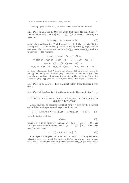
Thus, applying Theorem 3, we arrive at the assertion of Theorem 1.
5.2. Proof of Theorem 2. One can verify that under the conditions (9),
(10) the operators φ i : D([a, b], R n ) → L 1 ([a, b], R n ), i = 0, 1, defined by the
formulae
φ 0 := −θg 1 , φ 1 := g 0 + (1 − θ)g 1 (17)
satisfy the conditions (6), (7) of Theorem 1. Indeed, the estimate (9), the
assumption θ ∈ (0, 1), and the positivity of the operator g 1 imply that for
any absolutely continuous functions u = (u k ) n k=1 and v = (v k) n k=1
with the
properties (8) the relations
∣ (fk u)(t) − (f k v)(t) + θg 1 (u − v)(t) ∣ =
= ∣ ∣ (fk u)(t) − (f k v)(t) + g 1k (u − v)(t) − (1 − θ)g 1k (u − v)(t) ∣ ∣ ≤
≤ g 0k (u − v)(t) + ∣ ∣ (1 − θ)g1k (u − v)(t) ∣ ∣ =
= g 0k (u − v)(t) + (1 − θ)(g 1k (u − v)(t)), t ∈ [a, b], k = 1, 2, . . . , n,
are true. This means that f admits the estimate (7) with the operators φ 0
and φ 1 defined by the formulae (17). Therefore, it remains only to note
that the assumption (10) ensures the validity of the inclusions (6) for the
operators (17). Applying Theorem 1, we arrive at the required assertion.
5.3. Proof of Corollary 1. This statement follows from Theorem 2 with
θ = 1 2 .
5.4. Proof of Corollary 2. It is sufficient to apply Theorem 2 with θ = 1 4 .
6. Example of a Scalar Nonlinear Differential Equation with
Argument Deviations
As an example, we consider the initial value problem for the nonlinear
scalar differential equation with argument deviations
u ′ (t) = µ 0 (t) √ 1 + λ(t) sin u(ω 0 (t)) − µ 1 (t)u(ω 1 (t)), t ∈ [a, b], (18)
with the initial condition
u(a) = c, (19)
where c ∈ R is an arbitrary constant, ω i : [a, b] → [a, b], i = 0, 1, are
Lebesgue measurable functions, and {λ, µ i } ⊂ L 1 ([a, b], R), i = 0, 1, are
functions such that
0 ≤ λ(t) < 1 for a.e. t ∈ [a, b]. (20)
It is important to point out that the first term in (18) may not be of
retarding type (i.e., the set {t ∈ [a, b] : ω 0 (t) > t} may have non-zero measure)
and, therefore, the solvability of the problem (18), (19) is not obvious.