CHAPTER 8: MATRICES and DETERMINANTS - Kkuniyuk.com
CHAPTER 8: MATRICES and DETERMINANTS - Kkuniyuk.com CHAPTER 8: MATRICES and DETERMINANTS - Kkuniyuk.com
(Section 8.1: Matrices and Determinants) 8.01 CHAPTER 8: MATRICES and DETERMINANTS The material in this chapter will be covered in your Linear Algebra class (Math 254 at Mesa). SECTION 8.1: MATRICES and SYSTEMS OF EQUATIONS PART A: MATRICES A matrix is basically an organized box (or “array”) of numbers (or other expressions). In this chapter, we will typically assume that our matrices contain only numbers. Example Here is a matrix of size 2 3 (“2 by 3”), because it has 2 rows and 3 columns: 1 0 2 0 1 5 The matrix consists of 6 entries or elements. In general, an m n matrix has m rows and n columns and has mn entries. Example Here is a matrix of size 2 2 (an order 2 square matrix): 4 1 3 2 The boldfaced entries lie on the main diagonal of the matrix. (The other diagonal is the skew diagonal.)
- Page 2 and 3: (Section 8.1: Matrices and Determin
- Page 4 and 5: PART C: ELEMENTARY ROW OPERATIONS (
- Page 6 and 7: (Section 8.1: Matrices and Determin
- Page 8 and 9: (Section 8.1: Matrices and Determin
- Page 10 and 11: (Section 8.1: Matrices and Determin
- Page 12 and 13: (Section 8.1: Matrices and Determin
- Page 14 and 15: Step 4) Use back-substitution. (Sec
- Page 16 and 17: (Section 8.1: Matrices and Determin
- Page 18 and 19: Now, write down the new matrix: (Se
- Page 20 and 21: (Section 8.1: Matrices and Determin
- Page 22 and 23: (Section 8.1: Matrices and Determin
- Page 24 and 25: PART F: ROW-ECHELON FORM FOR A MATR
- Page 26 and 27: (Section 8.1: Matrices and Determin
- Page 28 and 29: (Section 8.1: Matrices and Determin
- Page 30 and 31: (Section 8.1: Matrices and Determin
- Page 32 and 33: Now for some steps we haven’t see
- Page 34 and 35: (Section 8.2: Operations with Matri
- Page 36 and 37: (Section 8.2: Operations with Matri
- Page 38 and 39: PART D : ( A ROW VECTOR) TIMES ( A
- Page 40 and 41: (Section 8.2: Operations with Matri
- Page 42 and 43: (Section 8.2: Operations with Matri
- Page 44 and 45: (Section 8.2: Operations with Matri
- Page 46 and 47: (Section 8.2: Operations with Matri
- Page 48 and 49: (Section 8.3: The Inverse of a Squa
- Page 50 and 51: (Section 8.3: The Inverse of a Squa
(Section 8.1: Matrices <strong>and</strong> Determinants) 8.01<br />
<strong>CHAPTER</strong> 8: <strong>MATRICES</strong> <strong>and</strong> <strong>DETERMINANTS</strong><br />
The material in this chapter will be covered in your Linear Algebra class (Math 254 at Mesa).<br />
SECTION 8.1: <strong>MATRICES</strong> <strong>and</strong> SYSTEMS OF EQUATIONS<br />
PART A: <strong>MATRICES</strong><br />
A matrix is basically an organized box (or “array”) of numbers (or other expressions).<br />
In this chapter, we will typically assume that our matrices contain only numbers.<br />
Example<br />
Here is a matrix of size 2 3 (“2 by 3”), because it has 2 rows <strong>and</strong> 3 columns:<br />
1 0 2<br />
<br />
0 1 5<br />
The matrix consists of 6 entries or elements.<br />
In general, an m n matrix has m rows <strong>and</strong> n columns <strong>and</strong> has mn entries.<br />
Example<br />
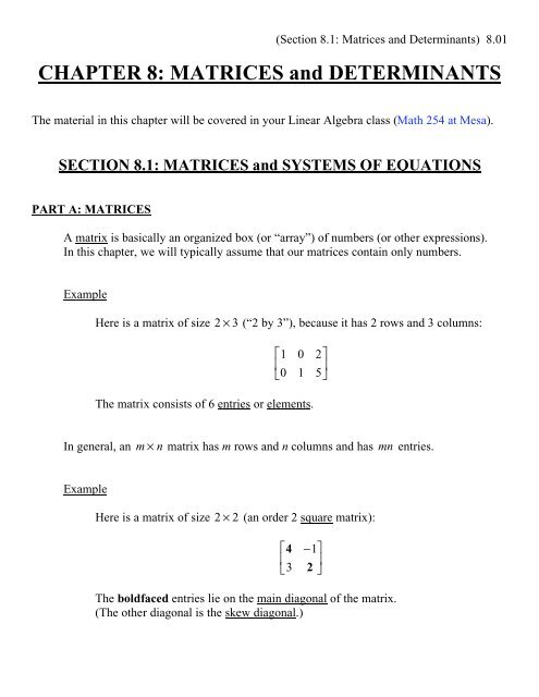
Here is a matrix of size 2 2 (an order 2 square matrix):<br />
4 1<br />
<br />
3 2 <br />
The boldfaced entries lie on the main diagonal of the matrix.<br />
(The other diagonal is the skew diagonal.)
(Section 8.1: Matrices <strong>and</strong> Determinants) 8.02<br />
PART B: THE AUGMENTED MATRIX FOR A SYSTEM OF LINEAR EQUATIONS<br />
Example<br />
Write the augmented matrix for the system:<br />
3x + 2y + z = 0<br />
<br />
2x z = 3<br />
Solution<br />
Preliminaries:<br />
Make sure that the equations are in (what we refer to now as)<br />
st<strong>and</strong>ard form, meaning that …<br />
• All of the variable terms are on the left side (with x, y, <strong>and</strong> z<br />
ordered alphabetically), <strong>and</strong><br />
• There is only one constant term, <strong>and</strong> it is on the right side.<br />
Line up like terms vertically.<br />
Here, we will rewrite the system as follows:<br />
3x + 2y + z = 0<br />
<br />
2x z = 3<br />
(Optional) Insert “1”s <strong>and</strong> “0”s to clarify coefficients.<br />
3x + 2y + 1z = 0<br />
<br />
2x + 0y 1z = 3<br />
Warning: Although this step is not necessary, people often<br />
mistake the coefficients on the z terms for “0”s.
(Section 8.1: Matrices <strong>and</strong> Determinants) 8.03<br />
Write the augmented matrix:<br />
Coefficients of Right<br />
x y z sides<br />
<br />
<br />
<br />
3 2 1<br />
2 0 1<br />
0<br />
3<br />
<br />
<br />
<br />
Coefficient matrix<br />
Right-h<strong>and</strong><br />
side (RHS)<br />
<br />
Augmented matrix<br />
We may refer to the first three columns as the x-column, the<br />
y-column, <strong>and</strong> the z-column of the coefficient matrix.<br />
Warning: If you do not insert “1”s <strong>and</strong> “0”s, you may want to read the<br />
equations <strong>and</strong> fill out the matrix row by row in order to minimize the<br />
chance of errors. Otherwise, it may be faster to fill it out column by<br />
column.<br />
The augmented matrix is an efficient representation of a system of<br />
linear equations, although the names of the variables are hidden.
PART C: ELEMENTARY ROW OPERATIONS (EROs)<br />
(Section 8.1: Matrices <strong>and</strong> Determinants) 8.04<br />
Recall from Algebra I that equivalent equations have the same solution set.<br />
Example<br />
Solve: 2x 1 = 5<br />
2x 1 = 5<br />
2x = 6<br />
x = 3 Solution set is {}. 3<br />
To solve the first equation, we write a sequence of equivalent equations until<br />
we arrive at an equation whose solution set is obvious.<br />
The steps of adding 1 to both sides of the first equation <strong>and</strong> of dividing both<br />
sides of the second equation by 2 are like “legal chess moves” that allowed<br />
us to maintain equivalence (i.e., to preserve the solution set).<br />
Similarly, equivalent systems have the same solution set.<br />
Elementary Row Operations (EROs) represent the legal moves that allow us to write a<br />
sequence of row-equivalent matrices (corresponding to equivalent systems) until we<br />
obtain one whose corresponding solution set is easy to find. There are three types of<br />
EROs:
(Section 8.1: Matrices <strong>and</strong> Determinants) 8.05<br />
1) Row Reordering<br />
Example<br />
Consider the system:<br />
3x y = 1<br />
<br />
x + y = 4<br />
If we switch (i.e., interchange) the two equations, then the solution set<br />
is not disturbed:<br />
x + y = 4<br />
<br />
3x y = 1<br />
This suggests that, when we solve a system using augmented matrices,<br />
…<br />
We can switch any two rows.<br />
Before:<br />
R 1<br />
3 1<br />
<br />
R 2 1 1<br />
1<br />
<br />
4<br />
Here, we switch rows R 1<br />
<strong>and</strong> R 2<br />
, which we denote<br />
by: R 1<br />
R 2<br />
After:<br />
new R 1<br />
1 1<br />
<br />
new R 2 3 1<br />
4<br />
<br />
1<br />
In general, we can reorder the rows of an augmented matrix<br />
in any order.<br />
Warning: Do not reorder columns; in the coefficient matrix,<br />
that will change the order of the corresponding variables.
(Section 8.1: Matrices <strong>and</strong> Determinants) 8.06<br />
2) Row Rescaling<br />
Example<br />
Consider the system:<br />
1<br />
<br />
2 x + 1 2 y = 3<br />
<br />
y = 4<br />
If we multiply “through” both sides of the first equation by 2, then we<br />
obtain an equivalent equation <strong>and</strong>, overall, an equivalent system:<br />
x + y = 6<br />
<br />
y = 4<br />
This suggests that, when we solve a system using augmented matrices,<br />
…<br />
We can multiply (or divide) “through” a row by any<br />
nonzero constant.<br />
Before:<br />
R 1<br />
1/2 1/2<br />
<br />
R 2 0 1<br />
3<br />
<br />
4<br />
Here, we multiply through R 1<br />
by 2, which we<br />
denote by: R 1<br />
2 R 1<br />
, or ( new R 1 ) 2 old R 1<br />
( )<br />
After:<br />
new R 1<br />
1 1<br />
<br />
R 2 0 1<br />
6<br />
<br />
4
(Section 8.1: Matrices <strong>and</strong> Determinants) 8.07<br />
3) Row Replacement<br />
(This is perhaps poorly named, since ERO types 1 <strong>and</strong> 2 may also be viewed<br />
as “row replacements” in a literal sense.)<br />
When we solve a system using augmented matrices, …<br />
Example<br />
We can add a multiple of one row to another row.<br />
Technical Note: This <strong>com</strong>bines ideas from the Row Rescaling ERO<br />
<strong>and</strong> the Addition Method from Chapter 7.<br />
Consider the system:<br />
<br />
<br />
<br />
x + 3y = 3<br />
2x + 5y = 16<br />
Before:<br />
R 1<br />
1 3<br />
<br />
R 2 2 5<br />
3 <br />
<br />
16<br />
Note: We will sometimes boldface items for purposes of clarity.<br />
It turns out that we want to add twice the first row to the second<br />
row, because we want to replace the “ 2 ” with a “0.”<br />
We denote this by:<br />
R 2<br />
R 2<br />
+ 2 R 1<br />
, or ( new R 2 ) ( old R 2 )+ 2 R 1<br />
old R 2<br />
2 5 16<br />
+ 2 R 1<br />
2 6 6<br />
new R 2<br />
0 11 22
(Section 8.1: Matrices <strong>and</strong> Determinants) 8.08<br />
Warning: It is highly advised that you write out the table!<br />
People often rush through this step <strong>and</strong> make mechanical errors.<br />
Warning: Although we can also subtract a multiple of one row<br />
from another row, we generally prefer to add, instead, even if<br />
that means that we multiply “through” a row by a negative<br />
number. Errors are <strong>com</strong>mon when people subtract.<br />
After:<br />
old R 1<br />
1 3<br />
<br />
new R 2 0 11<br />
3 <br />
<br />
22<br />
Note: In principle, you could replace the old R 1<br />
with the<br />
rescaled version, but it turns out that we like having that “1” in<br />
the upper left h<strong>and</strong> corner!<br />
If matrix B is obtained from matrix A after applying one or more EROs, then we<br />
call A <strong>and</strong> B row-equivalent matrices, <strong>and</strong> we write A B .<br />
Example<br />
1 2<br />
<br />
7 8<br />
3<br />
<br />
9<br />
<br />
7 8<br />
<br />
1 2<br />
9<br />
<br />
3<br />
Row-equivalent augmented matrices correspond to equivalent systems, assuming<br />
that the underlying variables (corresponding to the columns of the coefficient<br />
matrix) stay the same <strong>and</strong> are in the same order.
(Section 8.1: Matrices <strong>and</strong> Determinants) 8.09<br />
PART D: GAUSSIAN ELIMINATION (WITH BACK-SUBSTITUTION)<br />
This is a method for solving systems of linear equations.<br />
Historical Note: This method was popularized by the great mathematician Carl Gauss,<br />
but the Chinese were using it as early as 200 BC.<br />
Steps<br />
Given a square system (i.e., a system of n linear equations in n unknowns for some<br />
n Z + ; we will consider other cases later) …<br />
1) Write the augmented matrix.<br />
2) Use EROs to write a sequence of row-equivalent matrices until you get one in<br />
the form:<br />
If we begin with a square system, then all of the coefficient matrices will be<br />
square.<br />
We want “1”s along the main diagonal <strong>and</strong> “0”s all below.<br />
The other entries are “wild cards” that can potentially be any real numbers.<br />
This is the form that we are aiming for. Think of this as “checkmate” or<br />
“the top of the jigsaw puzzle box” or “the TARGET” (like in a trig ID).<br />
Warning: As you perform EROs <strong>and</strong> this form crystallizes <strong>and</strong> emerges,<br />
you usually want to avoid “undoing” the good work you have already done.<br />
For example, if you get a “1” in the upper left corner, you usually want to<br />
preserve it. For this reason, it is often a good strategy to “correct” the<br />
columns from left to right (that is, from the leftmost column to the<br />
rightmost column) in the coefficient matrix. Different strategies may work<br />
better under different circumstances.
(Section 8.1: Matrices <strong>and</strong> Determinants) 8.10<br />
For now, assume that we have succeeded in obtaining this form; this<br />
means that the system has exactly one solution.<br />
What if it is impossible for us to obtain this form? We shall discuss this<br />
matter later (starting with Notes 8.21).<br />
3) Write the new system, <strong>com</strong>plete with variables.<br />
This system will be equivalent to the given system, meaning that they share<br />
the same solution set. The new system should be easy to solve if you …<br />
4) Use back-substitution to find the values of the unknowns.<br />
We will discuss this later.<br />
5) Write the solution as an ordered n-tuple (pair, triple, etc.).<br />
6) Check the solution in the given system. (Optional)<br />
Warning: This check will not capture other solutions if there are, in fact,<br />
infinitely many solutions.<br />
Technical Note: This method actually works with <strong>com</strong>plex numbers in general.<br />
Warning: You may want to quickly check each of your steps before proceeding. A single<br />
mistake can have massive consequences that are difficult to correct.
(Section 8.1: Matrices <strong>and</strong> Determinants) 8.11<br />
Example<br />
4x y = 13<br />
Solve the system: <br />
x 2y = 5<br />
Solution<br />
Step 1) Write the augmented matrix.<br />
You may first want to insert “1”s <strong>and</strong> “0”s where appropriate.<br />
4x 1y = 13<br />
<br />
1x 2y = 5<br />
R 1<br />
4 1<br />
<br />
R 2 1 2<br />
13<br />
<br />
5 <br />
Note: It’s up to you if you want to write the “ R 1<br />
” <strong>and</strong> the “ R 2<br />
.”<br />
Step 2) Use EROs until we obtain the desired form:<br />
1 ?<br />
<br />
0 1<br />
? <br />
<br />
? <br />
Note: There may be different “good” ways to achieve our goal.<br />
We want a “1” to replace the “4” in the upper left.<br />
Dividing through R 1<br />
by 4 will do it, but we will then end up with<br />
fractions. Sometimes, we can’t avoid fractions. Here, we can.<br />
Instead, let’s switch the rows.<br />
R 1<br />
R 2<br />
Warning: You should keep a record of your EROs. This will reduce<br />
eyestrain <strong>and</strong> frustration if you want to check your work!<br />
R 1<br />
1 2<br />
<br />
R 2 4 1<br />
5 <br />
<br />
13
(Section 8.1: Matrices <strong>and</strong> Determinants) 8.12<br />
We now want a “0” to replace the “4” in the bottom left.<br />
Remember, we generally want to “correct” columns from left to right,<br />
so we will attack the position containing the 1 later.<br />
We cannot multiply through a row by 0.<br />
Instead, we will use a row replacement ERO that exploits the “1” in<br />
the upper left to “kill off” the “4.” This really represents the<br />
elimination of the x term in what is now the second equation in our<br />
system.<br />
( new R 2 ) ( old R 2 )+ ( 4) R 1<br />
The notation above is really unnecessary if you show the work below:<br />
old R 2<br />
4 1 13<br />
+ ( 4) R 1<br />
4 8 20<br />
new R 2<br />
0 7 7<br />
R 1<br />
1 2<br />
<br />
R 2 0 7<br />
5 <br />
<br />
7<br />
We want a “1” to replace the “7.”<br />
We will divide through R 2<br />
by 7, or, equivalently, we will multiply<br />
through R 2<br />
by 1 7 :<br />
R 2<br />
1 7 R 2 , or<br />
R 1<br />
1 2<br />
<br />
R 2 0 7<br />
5 <br />
<br />
7<br />
÷ 7<br />
R 1<br />
1 2<br />
<br />
R 2 0 1<br />
5 <br />
<br />
1
We now have our desired form.<br />
(Section 8.1: Matrices <strong>and</strong> Determinants) 8.13<br />
Technical Note: What’s best for <strong>com</strong>putation by h<strong>and</strong> may not be best<br />
for <strong>com</strong>puter algorithms that attempt to maximize precision <strong>and</strong><br />
accuracy. For example, the strategy of partial pivoting would have<br />
kept the “4” in the upper left position of the original matrix <strong>and</strong> would<br />
have used it to eliminate the “1” below.<br />
Note: Some books remove the requirement that the entries along the<br />
main diagonal all have to be “1”s. However, when we refer to<br />
Gaussian Elimination, we will require that they all be “1”s.<br />
Step 3) Write the new system.<br />
You may want to write down the variables on top of their<br />
corresponding columns.<br />
x y<br />
1 2<br />
<br />
0 1<br />
5 <br />
<br />
1<br />
x 2y = 5<br />
<br />
y = 1<br />
<br />
This is called an upper triangular system, which is very easy to solve<br />
if we …
Step 4) Use back-substitution.<br />
(Section 8.1: Matrices <strong>and</strong> Determinants) 8.14<br />
We start at the bottom, where we immediately find that y = 1.<br />
We then work our way up the system, plugging in values for<br />
unknowns along the way whenever we know them.<br />
x 2y = 5<br />
x 2( 1)= 5<br />
x + 2 = 5<br />
x =3<br />
Step 5) Write the solution.<br />
The solution set is:<br />
{( 3, 1)<br />
}.<br />
Books are often content with omitting the { } brace symbols.<br />
Ask your instructor, though.<br />
Warning: Observe that the order of the coordinates is the reverse of<br />
the order in which we found them in the back-substitution procedure.<br />
Step 6) Check. (Optional)<br />
Given system:<br />
4x y = 13<br />
<br />
x 2y = 5<br />
<br />
43<br />
( ) ( 1)= 13<br />
<br />
( 3) 2( 1)= 5<br />
13 = 13<br />
<br />
5 = 5<br />
Our solution checks out.
(Section 8.1: Matrices <strong>and</strong> Determinants) 8.15<br />
Example (#62 on p.556)<br />
Solve the system:<br />
2x + 2y z = 2<br />
<br />
x 3y + z = 28<br />
<br />
x + y = 14<br />
Solution<br />
Step 1) Write the augmented matrix.<br />
You may first want to insert “1”s <strong>and</strong> “0”s where appropriate.<br />
2x + 2y 1z = 2<br />
<br />
1x 3y + 1z = 28<br />
<br />
1x + 1y + 0z = 14<br />
R 1<br />
2 2 1<br />
<br />
R 2 1 3 1<br />
R <br />
3 <br />
1 1 0<br />
2 <br />
<br />
28<br />
14 <br />
<br />
Step 2) Use EROs until we obtain the desired form:<br />
1 ? ?<br />
<br />
0 1 ?<br />
<br />
<br />
0 0 1<br />
? <br />
<br />
? <br />
? <br />
<br />
We want a “1” to replace the “2” in the upper left corner.<br />
Dividing through R 1<br />
by 2 would do it, but we would then end up<br />
with a fraction.<br />
Instead, let’s switch the first two rows.<br />
R 1<br />
R 2
(Section 8.1: Matrices <strong>and</strong> Determinants) 8.16<br />
R 1<br />
1 3 1<br />
<br />
R 2 2 2 1<br />
R <br />
3 <br />
1 1 0<br />
28<br />
<br />
2 <br />
14 <br />
<br />
We now want to “eliminate down” the first column by using the “1”<br />
in the upper left corner to “kill off” the boldfaced entries <strong>and</strong> turn<br />
them into “0”s.<br />
Warning: Performing more than one ERO before writing down a new<br />
matrix often risks mechanical errors. However, when eliminating<br />
down a column, we can usually perform several row replacement<br />
EROs without confusion before writing a new matrix. (The same is<br />
true of multiple row rescalings <strong>and</strong> of row reorderings, which can<br />
represent multiple row interchanges.) Mixing ERO types before<br />
writing a new matrix is probably a bad idea, though!<br />
old R 2<br />
2 2 1 2<br />
+ ( 2) R 1<br />
2 6 2 56<br />
new R 2<br />
0 8 3 58<br />
old R 3<br />
1 1 0 14<br />
+R 1<br />
1 3 1 28<br />
new R 3<br />
0 2 1 14<br />
Now, write down the new matrix:<br />
R 1<br />
1 3 1<br />
<br />
R 2 0 8 3<br />
R <br />
3 <br />
0 2 1<br />
28<br />
<br />
58 <br />
14<br />
<br />
The first column has been “corrected.” From a strategic perspective,<br />
we may now think of the first row <strong>and</strong> the first column (in blue) as<br />
“locked in.” (EROs that change the entries therein are not necessarily<br />
“wrong,” but you may be in danger of being taken further away from<br />
the desired form.)
(Section 8.1: Matrices <strong>and</strong> Determinants) 8.17<br />
We will now focus on the second column. We want:<br />
1 3 1<br />
<br />
0 1 ?<br />
<br />
<br />
0 0 ?<br />
28<br />
<br />
? <br />
? <br />
<br />
Here is our current matrix:<br />
R 1<br />
1 3 1<br />
<br />
R 2 0 8 3<br />
R <br />
3 <br />
0 2 1<br />
28<br />
<br />
58 <br />
14<br />
<br />
If we use the “ 2 ” to kill off the “8,” we can avoid fractions for the<br />
time being. Let’s first switch R 2<br />
<strong>and</strong> R 3<br />
so that we don’t get confused<br />
when we do this. (We’re used to eliminating down a column.)<br />
Technical Note: The <strong>com</strong>puter-based strategy of partial pivoting<br />
would use the “8” to kill off the “ 2 ,” since the “8” is larger in<br />
absolute value.<br />
R 2<br />
R 3<br />
R 1<br />
1 3 1<br />
<br />
R 2 0 2 1<br />
R <br />
3 <br />
0 8 3<br />
28<br />
<br />
14<br />
58 <br />
<br />
Now, we will use a row replacement ERO to eliminate the “8.”<br />
old R 3<br />
0 8 3 58<br />
+ 4 R 2<br />
0 8 4 56<br />
new R 3<br />
0 0 1 2<br />
Warning: Don’t ignore the “0”s on the left; otherwise, you may get<br />
confused.
Now, write down the new matrix:<br />
(Section 8.1: Matrices <strong>and</strong> Determinants) 8.18<br />
R 1<br />
1 3 1<br />
<br />
R 2 0 2 1<br />
R <br />
3 <br />
0 0 1<br />
28<br />
<br />
14<br />
2 <br />
<br />
Once we get a “1” where the “ 2 ” is, we’ll have our desired form.<br />
We are fortunate that we already have a “1” at the bottom of the third<br />
column, so we won’t have to “correct” it.<br />
We will divide through R 2<br />
by 2, or, equivalently, we will multiply<br />
through R 2<br />
by 1 2 . R 2<br />
1 2<br />
<br />
<br />
<br />
<br />
<br />
R , or 2<br />
R 1<br />
1 3 1<br />
<br />
R 2 0 2 1<br />
R <br />
3 <br />
0 0 1<br />
28<br />
<br />
14<br />
2 <br />
<br />
÷ ( 2)<br />
We finally obtain a matrix in our desired form:<br />
R 1<br />
1 3 1<br />
<br />
R 2 0 1 1/2<br />
R <br />
3 <br />
0 0 1<br />
28<br />
<br />
7 <br />
2
Step 3) Write the new system.<br />
(Section 8.1: Matrices <strong>and</strong> Determinants) 8.19<br />
x y z<br />
1 3 1<br />
<br />
0 1 1/2<br />
<br />
<br />
0 0 1<br />
28<br />
<br />
7 <br />
2 <br />
<br />
x 3y + z = 28<br />
<br />
y 1 2 z = 7<br />
<br />
<br />
z = 2<br />
<br />
<br />
Step 4) Use back-substitution.<br />
We immediately have: z =2<br />
Use z = 2 in the second equation:<br />
y 1 2 z = 7<br />
y 1 (<br />
2 2 )= 7<br />
y 1 = 7<br />
y =8<br />
Use y = 8 <strong>and</strong> z = 2 in the first equation:<br />
x 3y + z = 28<br />
x 38 ( )+ ( 2)= 28<br />
x 24 + 2 = 28<br />
x 22 = 28<br />
x = 6
(Section 8.1: Matrices <strong>and</strong> Determinants) 8.20<br />
Step 5) Write the solution.<br />
The solution set is: {( 6, 8, 2)<br />
}.<br />
Warning: Remember that the order of the coordinates is the reverse of<br />
the order in which we found them in the back-substitution procedure.<br />
Step 6) Check. (Optional)<br />
Given system:<br />
2x + 2y z = 2<br />
<br />
x 3y + z = 28<br />
<br />
x + y = 14<br />
2( 6)+ 28 ( ) ( 2)= 2<br />
<br />
( 6) 38 ( )+ ( 2)= 28<br />
<br />
<br />
6 ( )+ ( 8) = 14<br />
2 = 2<br />
<br />
28 = 28<br />
<br />
14 = 14<br />
Our solution checks out.
PART E: WHEN DOES A SYSTEM HAVE NO SOLUTION?<br />
(Section 8.1: Matrices <strong>and</strong> Determinants) 8.21<br />
If we ever get a row of the form:<br />
0 0 0 ( non-0 constant),<br />
then STOP! We know at this point that the solution set is .<br />
Example<br />
Solve the system:<br />
x + y = 1<br />
<br />
x + y = 4<br />
Solution<br />
The augmented matrix is:<br />
R 1<br />
1 1<br />
<br />
R 2 1 1<br />
1<br />
<br />
4<br />
We can quickly subtract R 1<br />
from R 2<br />
. We then obtain:<br />
R 1<br />
1 1<br />
<br />
R 2 0 0<br />
1<br />
<br />
3<br />
The new R 2<br />
implies that the solution set is .<br />
Comments: This is because R 2<br />
corresponds to the equation 0 = 3, which<br />
cannot hold true for any pair ( x, y).
(Section 8.1: Matrices <strong>and</strong> Determinants) 8.22<br />
If we get a row of all “0”s, such as:<br />
0 0 0 0 ,<br />
then what does that imply? The story is more <strong>com</strong>plicated here.<br />
Example<br />
Solve the system:<br />
x + y = 4<br />
<br />
x + y = 4<br />
Solution<br />
The augmented matrix is:<br />
R 1<br />
1 1<br />
<br />
R 2 1 1<br />
4<br />
<br />
4<br />
We can quickly subtract R 1<br />
from R 2<br />
. We then obtain:<br />
R 1<br />
1 1<br />
<br />
R 2 0 0<br />
4<br />
<br />
0<br />
The corresponding system is then:<br />
x + y = 4<br />
<br />
0 = 0<br />
The equation 0 = 0 is pretty easy to satisfy. All ordered pairs x, y ( )<br />
satisfy it. In principle, we could delete this equation from the system.<br />
However, we tend not to delete rows in an augmented matrix, even if<br />
they consist of nothing but “0”s. The idea of changing the size of a<br />
matrix creeps us out.
(Section 8.1: Matrices <strong>and</strong> Determinants) 8.23<br />
The solution set is:<br />
{( x, y) x + y = 4}<br />
The system has infinitely many solutions; they correspond to all of the<br />
points on the line x + y = 4 .<br />
However, a row of all “0”s does not automatically imply that the corresponding<br />
system has infinitely many solutions.<br />
Example<br />
Consider the augmented matrix:<br />
R 1<br />
0 0<br />
<br />
R 2 0 0<br />
1<br />
<br />
0<br />
Because of R 1<br />
, the corresponding system actually has no solution.<br />
See Notes 7.12 for a similar example.<br />
The augmented matrices we have seen in this Part are not row equivalent to any<br />
matrix of the form<br />
R 1<br />
1 ?<br />
<br />
R 2 0 1<br />
? <br />
.<br />
? <br />
There was no way to get that desired form using EROs.<br />
What form do we aim for, then?
PART F: ROW-ECHELON FORM FOR A MATRIX<br />
If it is impossible for us to obtain the form<br />
(Section 8.1: Matrices <strong>and</strong> Determinants) 8.24<br />
(maybe because our coefficient matrix isn’t even square), then what do we aim for?<br />
We aim for row-echelon form; in fact, the above form is a special case of row-echelon<br />
form.<br />
Properties of a Matrix in Row-Echelon Form<br />
1) If there are any “all-0” rows, then they must be at the bottom of the matrix.<br />
Aside from these “all-0” rows,<br />
2) Every row must have a “1” (called a “leading 1”) as its leftmost non-0 entry.<br />
3) The “leading 1”s must “flow down <strong>and</strong> to the right.”<br />
More precisely: The “leading 1” of a row must be in a column to the right of<br />
the “leading 1”s of all higher rows.<br />
Example<br />
The matrix below is in Row-Echelon Form:<br />
1 3 0 7 4<br />
<br />
0 0 0 1 9<br />
0 0 0 0 1<br />
<br />
<br />
0 0 0 0 0<br />
1<br />
<br />
2<br />
3<br />
<br />
0<br />
The “leading 1”s are boldfaced.<br />
The “1” in the upper right corner is not a “leading 1.”
(Section 8.1: Matrices <strong>and</strong> Determinants) 8.25<br />
PART G: REDUCED ROW-ECHELON (RRE) FORM FOR A MATRIX<br />
This is a special case of Row-Echelon Form.<br />
Properties of a Matrix in Reduced Row-Echelon (RRE) Form<br />
1-3) It is in Row-Echelon form. (See Part F.)<br />
4) Each “leading 1” has all “0”s elsewhere in its column.<br />
Property 4) leads us to eliminate up from the “leading 1”s.<br />
Recall the matrix in Row-Echelon Form that we just saw:<br />
1 3 0 7 4<br />
<br />
0 0 0 1 9<br />
0 0 0 0 1<br />
<br />
<br />
0 0 0 0 0<br />
1<br />
<br />
2<br />
3<br />
<br />
0<br />
In order to obtain RRE Form, we must use row replacement EROs to kill off the three<br />
entries in purple (the “7,” the “4,” <strong>and</strong> the “9”); we need “0”s in those positions.
(Section 8.1: Matrices <strong>and</strong> Determinants) 8.26<br />
PART H: GAUSS-JORDAN ELIMINATION<br />
This is a matrix-heavy alternative to Gaussian Elimination in which we use EROs to go<br />
all the way to RRE Form.<br />
A matrix of numbers can have infinitely many Row-Echelon Forms [that the matrix is<br />
row-equivalent to], but it has only one unique RRE Form.<br />
Technical Note: The popular MATLAB (“Matrix Laboratory”) software has an “rref”<br />
<strong>com</strong>m<strong>and</strong> that gives this unique RRE Form for a given matrix.<br />
In fact, we can efficiently use Gauss-Jordan Elimination to help us describe the solution<br />
set of a system of linear equations with infinitely many solutions.<br />
Example<br />
Let’s say we have a system that we begin to solve using Gaussian Elimination.<br />
Let’s say we obtain the following matrix in Row-Echelon Form:<br />
1 2 3<br />
<br />
0 1 3<br />
0 0 1<br />
<br />
<br />
0 0 0<br />
9<br />
<br />
5<br />
2<br />
<br />
0<br />
Before this Part, we would stop with the matrices <strong>and</strong> write out the corresponding<br />
system.<br />
In Gauss-Jordan Elimination, however, we’re not satisfied with just any Row-<br />
Echelon Form for our final augmented matrix. We dem<strong>and</strong> RRE Form.<br />
To obtain RRE Form, we must eliminate up from two of the “leading 1”s <strong>and</strong> kill<br />
off the three purple entries: the “ 2” <strong>and</strong> the two “3”s. We need “0”s in those<br />
positions.<br />
In Gaussian Elimination, we “corrected” the columns from left to right in order to<br />
preserve our good works. At this stage, however, when we eliminate up, we prefer<br />
to correct the columns from right to left so that we can take advantage of the “0”s<br />
we create along the way.
(Section 8.1: Matrices <strong>and</strong> Determinants) 8.27<br />
(Reminder:)<br />
R 1<br />
R 2<br />
1 2 3<br />
<br />
0 1 3<br />
R <br />
3<br />
0 0 1<br />
<br />
R 4 <br />
0 0 0<br />
9<br />
<br />
5<br />
2<br />
<br />
0<br />
Use row replacement EROs to eliminate the two “3”s in the third column.<br />
Observe that we use a “leading 1” from a lower row to kill off an entry from<br />
a higher row.<br />
old R 2<br />
0 1 3 5<br />
+ ( 3) R 3<br />
0 0 3 6<br />
new R 2<br />
0 1 0 1<br />
old R 1<br />
1 2 3 9<br />
+ ( 3) R 3<br />
0 0 3 6<br />
new R 1<br />
1 2 0 3<br />
New matrix:<br />
R 1<br />
R 2<br />
1 2 0<br />
<br />
0 1 0<br />
R <br />
3<br />
0 0 1<br />
<br />
R 4 <br />
0 0 0<br />
3 <br />
<br />
1<br />
2 <br />
<br />
0 <br />
Now, use a row replacement ERO to eliminate the “ 2” in the second<br />
column.<br />
old R 1<br />
1 2 0 3<br />
+ 2 R 2<br />
0 2 0 2<br />
new R 1<br />
1 0 0 1<br />
Observe that our “right to left” strategy has allowed us to use “0”s to<br />
our advantage.
(Section 8.1: Matrices <strong>and</strong> Determinants) 8.28<br />
Here is the final RRE Form:<br />
R 1<br />
R 2<br />
x y z<br />
1 0 0<br />
<br />
0 1 0<br />
R <br />
3<br />
0 0 1<br />
<br />
R 4 <br />
0 0 0<br />
1 <br />
<br />
1<br />
2 <br />
<br />
0 <br />
We can read off our solution now!<br />
Solution set: {( 1, 1, 2)<br />
}.<br />
x = 1<br />
<br />
y = 1<br />
<br />
z = 2<br />
As you can see, some work has been moved from the back-substitution stage<br />
(which is now deleted) to the ERO stage.
(Section 8.1: Matrices <strong>and</strong> Determinants) 8.29<br />
PART I: SYSTEMS WITH INFINITELY MANY SOLUTIONS (OPTIONAL?)<br />
Example<br />
Solve the system:<br />
x 2y + z + 5w = 3<br />
<br />
2x 4y + z + 7w = 5<br />
Warning: In fact, w is often considered to be the fourth coordinate of ordered<br />
4-tuples of the form x, y, z, w ( ).<br />
Solution<br />
The augmented matrix is:<br />
R 1<br />
1 2 1 5<br />
<br />
R 2 2 4 1 7<br />
3<br />
<br />
5<br />
Let’s first go to Row-Echelon Form, which is required in both Gaussian<br />
Elimination <strong>and</strong> Gauss-Jordan Elimination – that is, unless it is clear at some<br />
point that there is no solution.<br />
We will use a row replacement ERO <strong>and</strong> use the “1” in the upper left corner<br />
to kill off the “2” in the lower left corner <strong>and</strong> get a “0” in there.<br />
New matrix:<br />
old R 2<br />
2 4 1 7 5<br />
+ ( 2) R 1<br />
2 4 2 10 6<br />
new R 2<br />
0 0 1 3 1<br />
R 1<br />
1 2 1 5<br />
<br />
R 2 0 0 1 3<br />
3 <br />
<br />
1<br />
We now need a “1” where the boldfaced “ 1” is.
(Section 8.1: Matrices <strong>and</strong> Determinants) 8.30<br />
To obtain Row-Echelon Form, we multiply through R 2<br />
by ( 1):<br />
The “leading 1”s are boldfaced.<br />
( new R 2 )( 1) ( old R 2 )<br />
x y z w<br />
R 1<br />
1 2 1 5 3 <br />
<br />
<br />
R 2 0 0 1 3 1 <br />
RHS<br />
We first observe that the system is consistent, because of the following rule:<br />
An augmented matrix in Row-Echelon Form corresponds to an<br />
inconsistent system (i.e., a system with no solution) <br />
(if <strong>and</strong> only if) there is a “leading 1” in the RHS.<br />
In other words, it corresponds to a consistent system <br />
there are no “leading 1”s in the RHS.<br />
Warning: There is a “1” in our RHS here in our Example, but it is not<br />
a “leading 1.”<br />
Each of the variables that correspond to the columns of the coefficient<br />
matrix (here, x, y, z, <strong>and</strong> w) is either a basic variable or a free variable.<br />
A variable is called a basic variable <br />
It corresponds to a column that has a “leading 1.”<br />
A variable is called a free variable <br />
It corresponds to a column that does not have a “leading 1.”<br />
In this Example, x <strong>and</strong> z are basic variables, <strong>and</strong> y <strong>and</strong> w are free variables.
(Section 8.1: Matrices <strong>and</strong> Determinants) 8.31<br />
Let’s say our system of linear equations is consistent.<br />
If there are no free variables, then the system has only one solution.<br />
Otherwise, if there is at least one free variable, then the system has<br />
infinitely many solutions.<br />
At this point, we know that the system in our Example has infinitely many<br />
solutions.<br />
If we want to <strong>com</strong>pletely describe the solution set of a system with infinitely<br />
many solutions, then we should use Gauss-Jordan Elimination <strong>and</strong> take our<br />
matrix to RRE Form. We must kill off the “1” in purple below.<br />
Our RRE Form:<br />
The corresponding system:<br />
x y z w<br />
R 1<br />
1 2 1 5 3 <br />
<br />
<br />
R 2 0 0 1 3 1 <br />
RHS<br />
old R 1<br />
1 2 1 5 3<br />
+ ( 1) R 2<br />
0 0 1 3 1<br />
new R 1<br />
1 2 0 2 2<br />
x y z w<br />
R 1<br />
1 2 0 2 2 <br />
<br />
<br />
R 2 0 0 1 3 1 <br />
RHS<br />
x 2y + 2w = 2<br />
<br />
z + 3w = 1
Now for some steps we haven’t seen before.<br />
(Section 8.1: Matrices <strong>and</strong> Determinants) 8.32<br />
We will parameterize (or parametrize) the free variables:<br />
Let y = a,<br />
w = b,<br />
where the parameters a <strong>and</strong> b represent<br />
any pair of real numbers.<br />
Both of the parameters are allowed to “roam freely” over the reals.<br />
Let’s rewrite our system using these parameters:<br />
x 2a + 2b = 2<br />
<br />
z + 3b = 1<br />
This is a system consisting of two variables <strong>and</strong> two parameters.<br />
We then solve the equations for the basic variables, x <strong>and</strong> z:<br />
x = 2 + 2a 2b<br />
<br />
z = 1 3b<br />
Remember that y = a <strong>and</strong> w = b, so we have:<br />
x = 2 + 2a 2b<br />
y = a<br />
<br />
z = 1 3b<br />
<br />
w = b<br />
Note: In your Linear Algebra class (Math 254 at Mesa), you may want to<br />
line up like terms.
We can now write the solution set.<br />
Comments<br />
(Section 8.1: Matrices <strong>and</strong> Determinants) 8.33<br />
{( 2 + 2a 2b, a, 1 3b, b) a <strong>and</strong> b are real numbers}<br />
This set consists of infinitely many solutions, each corresponding to a<br />
different pair of choices for a <strong>and</strong> b.<br />
Some solutions:<br />
a b ( x, y, z, w )<br />
0 0 ( 2, 0, 1, 0 )<br />
4 7 ( 20, 4, 20, 7 )<br />
Because we have two parameters, the graph of the solution set is a<br />
2-dimensional plane existing in 4-dimensional space. Unfortunately,<br />
we can’t see this graph! Nevertheless, this is the kind of thinking you<br />
will engage in in your Linear Algebra class (Math 254 at Mesa)!
(Section 8.2: Operations with Matrices) 8.34<br />
SECTION 8.2: OPERATIONS WITH <strong>MATRICES</strong><br />
We will not discuss augmented matrices until Part G.<br />
For now, we will simply think of a matrix as a box of numbers.<br />
PART A: NOTATION<br />
The matrix A = <br />
<br />
a ij<br />
<br />
, meaning that A consists of entries labeled a ij<br />
number, <strong>and</strong> j is the column number.<br />
Example<br />
<br />
If A is 2 2 , then A = a a<br />
11 12<br />
<br />
<br />
<br />
a 21<br />
a 22 .<br />
, where i is the row<br />
Note: a 12<br />
<strong>and</strong> a 21<br />
are not necessarily equal. If they are, then we have a<br />
symmetric matrix, which is a square matrix that is symmetric about its main<br />
2 3<br />
diagonal. An example of a symmetric matrix is: <br />
3 7
(Section 8.2: Operations with Matrices) 8.35<br />
PART B: WHEN DOES A = B?<br />
Two matrices (say A <strong>and</strong> B) are equal <br />
They have the same size, <strong>and</strong> they have the same numbers (or expressions) in the same<br />
positions.<br />
Example<br />
Example<br />
Example<br />
1 2<br />
<br />
= 1 2 <br />
<br />
3 4<br />
3 4<br />
1 2<br />
<br />
3 4<br />
1 3 <br />
<br />
2 4<br />
If the matrix on the left is A, then the matrix on the right is A T<br />
(“A transpose”). For the two matrices, the rows of one are the columns of the<br />
other.<br />
<br />
0 1 0 1 <br />
The two matrices have different sizes.<br />
The matrix on the left is 1 2 .<br />
It may be seen as a row vector, since it consists of only 1 row.<br />
The matrix on the right is 2 1.<br />
It may be seen as a column vector, since it consists of only 1 column.<br />
Observe that the matrices are transposes of each other.<br />
Think About It: What kind of matrix is, in fact, equal to its transpose?
(Section 8.2: Operations with Matrices) 8.36<br />
PART C: BASIC OPERATIONS<br />
Matrix addition: If two or more matrices have the same size, then you add them by<br />
adding corresponding entries. If the matrices do not have the same size, then the sum is<br />
undefined.<br />
Matrix subtraction problems can be rewritten as matrix addition problems.<br />
Scalar multiplication: To multiply a matrix by a scalar (i.e., a real number in this class),<br />
you multiply each entry of the matrix by the scalar.<br />
Example<br />
If<br />
then …<br />
<br />
A = 2 0 1 <br />
<br />
1 3 2<br />
<br />
B = 0 0 0 <br />
<br />
0 0 0<br />
B is the 2 3 zero matrix, denoted by “0” or “0 23<br />
” – it is the additive<br />
identity for the set of 2 3 real matrices. However, when we refer to<br />
“identity matrices,” we typically refer to multiplicative identities,<br />
which we will discuss later.<br />
<br />
C = 1 2 0 <br />
<br />
0 1 3
(Section 8.2: Operations with Matrices) 8.37<br />
1) Find A + B + 2C<br />
2 0 1<br />
<br />
A + B + 2C = + 0 0 0 <br />
+ 2 1 2 0 <br />
<br />
1 3 2<br />
0 0 0<br />
<br />
0 1 3<br />
<br />
<br />
Perform matrix addition.<br />
<br />
= 2 0 1 <br />
+ 2 4 0 <br />
<br />
1 3 2<br />
0 2 6<br />
<br />
= 4 4 1 <br />
<br />
1 5 4<br />
Perform scalar multiplication<br />
2) Find A 5C<br />
A 5C = A + ( 5)C<br />
<br />
= 2 0 1 <br />
+ ( 5) 1 2 0 <br />
<br />
1 3 2<br />
0 1 3<br />
<br />
= 2 0 1 5 10 0 <br />
+ <br />
<br />
1 3 2<br />
0 5 15<br />
<br />
= 3 10 1 <br />
<br />
<br />
1 2 17
PART D : ( A ROW VECTOR) TIMES ( A COLUMN VECTOR)<br />
(Section 8.2: Operations with Matrices) 8.38<br />
We will deal with this basic multiplication problem before we go on to matrix<br />
multiplication in general.<br />
b 1<br />
<br />
<br />
b<br />
Let’s say we have a row vector a 1<br />
a 2<br />
a n<br />
<strong>and</strong> a column vector<br />
2 <br />
<br />
.<br />
<br />
<br />
b n <br />
Observe that they have the same number of entries; otherwise, our product will be<br />
undefined. This is how we multiply the row vector <strong>and</strong> the column vector (in that order);<br />
the resulting product may be viewed as either a scalar or a 1 1 matrix, depending on the<br />
context of the problem:<br />
b 1<br />
<br />
<br />
a 1<br />
b 1<br />
+ a 2<br />
b 2<br />
++ a n<br />
b n ( as a scalar)<br />
b<br />
a 1<br />
a 2<br />
a n<br />
<br />
2 <br />
<br />
= or<br />
<br />
a<br />
<br />
b n <br />
1<br />
b 1<br />
+ a 2<br />
b 2<br />
++ a n<br />
b n<br />
as a 1 1 matrix<br />
<br />
( )<br />
In words, we add the products of corresponding entries.<br />
This should remind you of the dot product of two vectors, which we saw in<br />
Section 6.4: Notes 6.28.<br />
Warning: A column vector times a row vector (in that order) gives you something very<br />
different, namely an n n matrix. We will see why in the next Part.<br />
Example<br />
4 <br />
<br />
1 0 3 5 <br />
<br />
1<br />
<br />
<br />
= 4 + 0 3<br />
= 1<br />
= ()4 1 ( )+ ( 0) ( 5)+ ( 3) ( 1)<br />
The product may also be written as 1 .
(Section 8.2: Operations with Matrices) 8.39<br />
PART E: MATRIX MULTIPLICATION (AB)<br />
When multiplying matrices, we do not simply multiply corresponding entries, although<br />
MATLAB does have an operation for that.<br />
Technical Definition (Optional?)<br />
(Bear in mind that the “tricks” that we will discuss later will make all of this easier<br />
to swallow.)<br />
Given two matrices A <strong>and</strong> B, the matrix product AB is defined <br />
The rows of A <strong>and</strong> the columns of B have the same “length” (i.e., number of<br />
entries).<br />
That is: ( the number of columns of A)= ( the number of rows of B)<br />
If AB is defined, then the entry in its i th row <strong>and</strong> j th<br />
for appropriate values of i <strong>and</strong> j.<br />
column equals:<br />
( the i th row of A) times ( the j th column of B)<br />
Another way of looking at this:<br />
If we let C = AB , where C = <br />
<br />
c ij<br />
<br />
, then:<br />
c ij<br />
= ( the i th row of A) times ( the j th column of B)<br />
for appropriate values of i <strong>and</strong> j.
(Section 8.2: Operations with Matrices) 8.40<br />
Example <strong>and</strong> Tricks<br />
Consider the matrix product<br />
4 1<br />
1 1 0<br />
<br />
<br />
2 1 3<br />
3 0 .<br />
<br />
<br />
1 2 <br />
<br />
A <br />
B<br />
Is AB defined? If so, what is its size?<br />
Let’s consider the sizes of A <strong>and</strong> B:<br />
A B<br />
2 3 3 2<br />
If the two boxed “inner numbers” are equal, then AB is defined, because:<br />
( the number of columns of A)= ( the number of rows of B),<br />
as specified in our Technical Definition.<br />
Warning: The two “outer numbers” (the “2”s here) need not be equal.<br />
The fact that they are means that the matrix will be square.<br />
The size of AB is given by the two “outer numbers” in order.<br />
Here, AB will be 2 2 .<br />
In general, if A is m n , <strong>and</strong> B is n p , then AB will be m p .<br />
The trick <strong>com</strong>ing up will help explain why.
(Section 8.2: Operations with Matrices) 8.41<br />
Find AB.<br />
We will use a “traffic intersection” model.<br />
To begin our trick, we will write B to the “northeast” (i.e., entirely<br />
above <strong>and</strong> to the right) of A.<br />
Draw thin lines (in blue below) through the rows of A <strong>and</strong> thin lines<br />
(in red below) through the columns of B so that all intersection points<br />
are shown. These intersection points correspond to the entries of AB.<br />
We can see immediately that the size of AB will be 2 2 .<br />
Warning: Make sure your lines are thin <strong>and</strong> are placed so that, for<br />
example, no “ ” signs or “1”s are written over.<br />
At each intersection point, we take the corresponding row of A <strong>and</strong> the<br />
corresponding column of B, <strong>and</strong> we multiply them as we did in<br />
Part D. (We are essentially taking the dot product of the two vectors<br />
whose lines intersect at that point.)<br />
c 11<br />
= ()4 1 ( )+ ( 1) ( 3)+ ( 0) ()= 1 4 3 + 0 = 1<br />
c 12<br />
= ()1 1 ( )+ ( 1) ( 0)+ ( 0) ( 2)= 1+ 0 + 0 = 1<br />
c 21<br />
= ( 2) ( 4)+ ()3 1 ( )+ ( 3) ()= 1 8 + 3 + 3 = 14<br />
c 22<br />
= ( 2) ( 1)+ ()0 1 ( )+ ( 3) ( 2)= 2 + 0 + 6 = 4<br />
<br />
Therefore, AB = 1 1 <br />
<br />
14 4<br />
.
(Section 8.2: Operations with Matrices) 8.42<br />
If the rows of A do not have the same length as the columns of B<br />
(so that dot products cannot be taken), then the matrix product AB is<br />
undefined.<br />
Observe that this is all consistent with the Technical Definition.<br />
Even though you may not have to use the c ij<br />
notation, it may be a<br />
good idea to show some work for partial credit purposes.<br />
Warning: Matrix multiplication is not <strong>com</strong>mutative. It is often the case that<br />
AB BA. In fact, one product may be defined, while the other is not.<br />
Think About It: When are AB <strong>and</strong> BA both defined?<br />
Why was matrix multiplication defined in this way? The answer lies in your Linear<br />
Algebra course (Math 254 at Mesa). The idea of “<strong>com</strong>positions of linear transformations”<br />
is key. You’ll see.
(Section 8.2: Operations with Matrices) 8.43<br />
PART F: IDENTITY <strong>MATRICES</strong> “I”<br />
An identity matrix I is a square matrix with the following form:<br />
We require “1”s along the main diagonal <strong>and</strong> “0”s everywhere else.<br />
Observe that this is a special RRE Form; this will <strong>com</strong>e up in Part G.<br />
More specifically, I n<br />
is the n n identity.<br />
Example<br />
1 0 0<br />
<br />
I 3<br />
= 0 1 0<br />
<br />
0 0 1<br />
<br />
These matrices are multiplicative identities. They play the role that “1” does in the set of<br />
real numbers. (Remember that zero matrices were additive identities.)<br />
If A is an n n matrix, then AI n<br />
= A , <strong>and</strong> I n<br />
A = A.<br />
Comment: Although matrix multiplication is not, in general, <strong>com</strong>mutative, it is true<br />
that an identity matrix “<strong>com</strong>mutes” with a matrix of the same size. You get the<br />
same product, regardless of the order of multiplication.<br />
Note: Even if A is not n n , it is possible that AI n<br />
or I n<br />
A is defined, in which<br />
case the result is A. For example:<br />
1 0<br />
4 5 =<br />
0 1<br />
4 5
(Section 8.2: Operations with Matrices) 8.44<br />
PART G: MATRIX NOTATION <strong>and</strong> SYSTEMS OF LINEAR EQUATIONS<br />
Example (#56 on p.570)<br />
Consider the system:<br />
x 1<br />
+ x 2<br />
3x 3<br />
= 9<br />
<br />
x 1<br />
+ 2x 2<br />
= 6<br />
<br />
x 1<br />
x 2<br />
+ x 3<br />
= 5<br />
Observe that this is a square system of linear equations; the number of<br />
equations (3) equals the number of unknowns (3).<br />
We can write this system as a matrix (or matrix-vector) equation, AX = B :<br />
1 1 3<br />
x 1<br />
9 <br />
<br />
<br />
1 2 0 x 2 = 6 <br />
<br />
1 1 1 <br />
x <br />
<br />
<br />
3 <br />
5<br />
<br />
<br />
A X B<br />
A is the coefficient matrix (<strong>and</strong> it is square), <strong>and</strong> B is the RHS.<br />
X may be thought of as a vector of variables or as a solution vector.<br />
We will use Gauss-Jordan Elimination on the augmented matrix <br />
<br />
A B<br />
<br />
for X. This is what we basically did in Section 8.1.<br />
to solve<br />
In order to save time, we will skip the steps that take us to Row-Echelon<br />
Form. Don’t do this in your own work, though!<br />
The symbol indicates row-equivalence, not equality.<br />
1 1 3<br />
<br />
<br />
A B<br />
= <br />
1 2 0<br />
<br />
<br />
1 1 1<br />
<br />
1 1 3<br />
<br />
0 1 1<br />
<br />
<br />
0 0 1<br />
9 <br />
<br />
6 <br />
5<br />
<br />
9 <br />
<br />
5 <br />
2
(Section 8.2: Operations with Matrices) 8.45<br />
There are actually infinitely many possible Row-Echelon Forms for <br />
<br />
A B<br />
;<br />
the last matrix is just one of them. However, there is only one RRE Form.<br />
Let’s find it. We proceed with Gauss-Jordan Elimination by eliminating up<br />
from the “leading 1”s.<br />
1 1 3<br />
<br />
0 1 1<br />
<br />
<br />
0 0 1<br />
9 <br />
<br />
5 <br />
2<br />
<br />
We eliminate up the third column:<br />
old R 2<br />
0 1 1 5<br />
+R 3<br />
0 0 1 2<br />
new R 2<br />
0 1 0 3<br />
old R 1<br />
1 1 3 9<br />
+ 3 R 3<br />
0 0 3 6<br />
new R 1<br />
1 1 0 3<br />
New matrix:<br />
1 1 0<br />
<br />
0 1 0<br />
<br />
<br />
0 0 1<br />
3 <br />
<br />
3 <br />
2<br />
<br />
We eliminate up the second column:<br />
old R 1<br />
1 1 0 3<br />
+ ( 1) R 2<br />
0 1 0 3<br />
new R 1<br />
1 0 0 0
(Section 8.2: Operations with Matrices) 8.46<br />
RRE Form:<br />
1 0 0<br />
<br />
0 1 0<br />
<br />
<br />
0 0 1<br />
0 <br />
<br />
3 <br />
2<br />
<br />
Observe that the coefficient matrix is I 3<br />
, the 3 3 identity.<br />
The corresponding system is pretty nifty:<br />
x 1<br />
= 0<br />
<br />
x 2<br />
= 3<br />
<br />
x 3<br />
= 2<br />
This immediately gives us our solution vector, X:<br />
0 <br />
<br />
X = 3 <br />
<br />
2<br />
<br />
In general, if AX = B represents a square system of linear equations that has<br />
exactly one solution, then the RRE Form of <br />
<br />
A B<br />
<br />
will be <br />
<br />
I X <br />
, where I<br />
is the identity matrix that is the same size as A. We simply grab our solution<br />
from the new RHS.
(Section 8.3: The Inverse of a Square Matrix) 8.47<br />
SECTION 8.3: THE INVERSE OF A SQUARE MATRIX<br />
PART A: (REVIEW) THE INVERSE OF A REAL NUMBER<br />
<br />
If a is a nonzero real number, then aa 1 = a 1 <br />
<br />
a<br />
= 1.<br />
a 1 , or 1 , is the multiplicative inverse of a, because its product with a is 1,<br />
a<br />
the multiplicative identity.<br />
Example<br />
<br />
3 1 <br />
<br />
3<br />
= 1, so 3 <strong>and</strong> 1 3<br />
are multiplicative inverses of each other.<br />
PART B: THE INVERSE OF A SQUARE MATRIX<br />
If A is a square n n matrix, sometimes there exists a matrix A 1 (“A inverse”) such that<br />
AA 1 = I n<br />
<strong>and</strong> A 1 A = I n<br />
.<br />
An invertible matrix <strong>and</strong> its inverse <strong>com</strong>mute with respect to matrix multiplication.<br />
Then, A is invertible (or nonsingular), <strong>and</strong> A 1 is unique.<br />
In this course, an invertible matrix is assumed to be square.<br />
Technical Note: A nonsquare matrix may have a left inverse matrix or a right<br />
inverse matrix that “works” on one side of the product <strong>and</strong> produces an identity<br />
matrix. They cannot be the same matrix, however.
(Section 8.3: The Inverse of a Square Matrix) 8.48<br />
PART C : FINDING A - 1<br />
We will discuss a shortcut for 2 2 matrices in Part F.<br />
Assume that A is a given n n (square) matrix.<br />
Example<br />
A is invertible Its RRE Form is the identity matrix I n<br />
(or simply I).<br />
It turns out that a sequence of EROs that takes you from an invertible matrix<br />
A down to I will also take you from I down to A 1 . (A good Linear Algebra<br />
book will have a proof for this.) We can use this fact to efficiently find A 1 .<br />
We construct <br />
<br />
A I <br />
<br />
. We say that A is in the “left square” of this matrix,<br />
<strong>and</strong> I is in the “right square.”<br />
We apply EROs to <br />
<br />
A I <br />
<br />
until we obtain the RRE Form <br />
<br />
I A 1 <br />
.<br />
That is, as soon as you obtain I in the left square, you grab the matrix in the<br />
right square as your A 1 .<br />
If you ever get a row of “0”s in the left square, then it will be impossible to<br />
obtain <br />
<br />
I A 1 <br />
<br />
, <strong>and</strong> A is noninvertible (or singular).<br />
Let’s go back to our A matrix from Section 8.2: Notes 8.44.<br />
Find A 1 .<br />
1 1 3<br />
<br />
<br />
A = 1 2 0 <br />
<br />
1 1 1
(Section 8.3: The Inverse of a Square Matrix) 8.49<br />
Solution<br />
We construct <br />
<br />
A I <br />
: 1 1 3<br />
<br />
<br />
1 2 0<br />
<br />
<br />
1 1 1<br />
1 0 0<br />
<br />
0 1 0<br />
0 0 1<br />
<br />
We perform Gauss-Jordan Elimination to take the left square down to I.<br />
The right square will be affected in the process, because we perform EROs<br />
on entire rows “all the way across.”<br />
We will show a couple of row replacement EROs, <strong>and</strong> then we will leave the<br />
remaining steps to you.<br />
We will kill off the purple entries <strong>and</strong> put “0”s in their places.<br />
old R 2<br />
1 2 0 0 1 0<br />
+R 1<br />
1 1 3 1 0 0<br />
new R 2<br />
0 3 3 1 1 0<br />
old R 3<br />
1 1 1 0 0 1<br />
+ ( 1) R 1<br />
1 1 3 1 0 0<br />
new R 3<br />
0 2 4 1 0 1<br />
New matrix:<br />
1 1 3<br />
<br />
0 3 3<br />
<br />
<br />
0 2 4<br />
1 0 0<br />
<br />
1 1 0<br />
1 0 1<br />
<br />
(Your turn! Keep going ….)
(Section 8.3: The Inverse of a Square Matrix) 8.50<br />
RRE Form:<br />
(Remember, this form is unique.)<br />
<br />
1 0 0<br />
<br />
0 1 0<br />
<br />
0 0 1<br />
<br />
<br />
<br />
I<br />
<br />
1/3 1/3 1 <br />
<br />
1/6 2/3 1/2 <br />
1/6 1/3 1/2<br />
<br />
<br />
<br />
A 1<br />
Check. (Optional)<br />
You can check that AA 1 = I . If that holds, then it is automatically<br />
true that A 1 A = I . (The right inverse <strong>and</strong> the left inverse of an<br />
invertible matrix must be the same. An invertible matrix must<br />
<strong>com</strong>mute with its inverse.)
(Section 8.3: The Inverse of a Square Matrix) 8.51<br />
PART D: THE INVERSE MATRIX METHOD FOR SOLVING SYSTEMS<br />
In Section 8.2: Notes 8.44, we expressed a system in the matrix form AX = B :<br />
1 1 3<br />
x 1<br />
9 <br />
<br />
<br />
1 2 0 x 2 = 6 <br />
<br />
1 1 1 <br />
x <br />
<br />
<br />
3 <br />
5<br />
<br />
<br />
A X B<br />
A should look familiar. In Part C, we found its inverse, A 1 .<br />
How can we express X directly in terms of A <strong>and</strong> B?<br />
Review from Algebra I (Optional)<br />
Let’s say we want to solve ax = b , where a 0 <strong>and</strong> a <strong>and</strong> b are real<br />
constants.<br />
ax = b<br />
1<br />
<br />
a<br />
a <br />
x =<br />
1 <br />
<br />
a<br />
b<br />
<br />
=1<br />
x = b a<br />
Because a 1 represents the multiplicative inverse of a, we can say that<br />
a 1 = 1 , <strong>and</strong> the steps can be rewritten as follows:<br />
a<br />
ax = b<br />
a 1 a x = a 1 b<br />
=1<br />
x = a 1 b
Solving the Matrix Equation AX = B<br />
Assume that A is invertible.<br />
(Section 8.3: The Inverse of a Square Matrix) 8.52<br />
Note: Even though 0 is the only real number that is noninvertible (in a<br />
multiplicative sense), there are many matrices other than zero matrices<br />
that are noninvertible.<br />
It is assumed that A, X, <strong>and</strong> B have “<strong>com</strong>patible” sizes. That is, AX is<br />
defined, <strong>and</strong> AX <strong>and</strong> B have the same size.<br />
The steps should look familiar:<br />
AX = B<br />
A 1 A<br />
X = A 1 B<br />
= I<br />
X = A 1 B<br />
The Inverse Matrix Method for Solving a System of Linear Equations<br />
If A is invertible, then the system AX = B has a unique solution<br />
given by X = A 1 B .
(Section 8.3: The Inverse of a Square Matrix) 8.53<br />
Comments<br />
• We must left multiply both sides of AX = B by A 1 . If we were to<br />
right multiply, then we would obtain AXA 1 = BA 1 ; both sides of<br />
that equation are undefined, unless A is 1 1. Remember that matrix<br />
multiplication is not <strong>com</strong>mutative. Although x = ba 1 would have<br />
been acceptable in our Algebra I discussion (because multiplication of<br />
real numbers is <strong>com</strong>mutative), X = BA 1 would be inappropriate<br />
here.<br />
• I is the identity matrix that is the same size as A. It plays the role that<br />
“1” did in our Algebra I discussion, because 1 was the multiplicative<br />
identity for the set of real numbers.<br />
• This result is of more theoretical significance than practical<br />
significance. The Gaussian Elimination (with Back-Substitution)<br />
method we discussed earlier is often more efficient than this inversebased<br />
process. However, X = A 1 B is good to know if you’re using<br />
software you’re not familiar with. Also, there’s an important category<br />
of matrices called orthogonal matrices, for which A 1 = A T ; this<br />
makes matters a whole lot easier, since A T is trivial to find.
(Section 8.3: The Inverse of a Square Matrix) 8.54<br />
Back to Our Example<br />
We will solve the system from Section 8.2: Notes 8.44 using this Inverse Matrix<br />
Method.<br />
Solution<br />
1 1 3<br />
x 1<br />
9 <br />
<br />
<br />
1 2 0 x 2 = 6 <br />
<br />
1 1 1 <br />
x <br />
<br />
<br />
3 <br />
5<br />
<br />
<br />
A X B<br />
It helps a lot that we’ve already found A 1 in Part C; that’s the bulk of the<br />
work.<br />
X = A 1 B<br />
1/3 1/3 1 9 <br />
<br />
<br />
= 1/6 2/3 1/2<br />
6 <br />
<br />
1/6 1/3 1/2<br />
<br />
<br />
5<br />
<br />
0 <br />
<br />
= 3 <br />
<br />
2<br />
<br />
This agrees with our result from the Gauss-Jordan Elimination method we<br />
used in Section 8.2: Notes 8.44-8.46.
(Section 8.3: The Inverse of a Square Matrix) 8.55<br />
PART E : THE DETERMINANT OF A 2 2 MATRIX ("BUTTERFLY RULE" )<br />
<br />
If A = <br />
a<br />
c<br />
b <br />
<br />
d<br />
, then the determinant of A, denoted by det( A) or A , is given by:<br />
det( A)= ad bc<br />
i.e., det( A)= ( product along main diagonal) ( product along skew diagonal)<br />
The following “butterfly” image may help you recall this formula.<br />
Warning: A should not be confused with absolute value notation.<br />
See Section 8.4.<br />
We will further discuss determinants in Section 8.4.
(Section 8.3: The Inverse of a Square Matrix) 8.56<br />
PART F : SHORTCUT FORMULA FOR THE INVERSE OF A 2 2 MATRIX<br />
<br />
If A = <br />
a<br />
c<br />
b <br />
<br />
d<br />
, then:<br />
<br />
1<br />
A 1 =<br />
det A<br />
( )<br />
d<br />
<br />
c<br />
b<br />
<br />
a <br />
If det( A)= 0 , then A 1 does not exist.<br />
Remember that we:<br />
Switch the entries along the main diagonal.<br />
Flip the signs on (i.e., take the opposite of) the entries along the skew<br />
diagonal.<br />
This formula is consistent with the method from Part C.<br />
Example<br />
<br />
If A = 1 2 <br />
<br />
3 4<br />
, find A 1 .<br />
<br />
Solution<br />
First off:<br />
Now:<br />
det( A)= ()4 1 ( ) ( 2) ( 3)<br />
= 2<br />
A 1 = 1 4 2<br />
<br />
2 3 1 <br />
<br />
= 2 1 <br />
<br />
3/2 1/2
(Section 8.4: The Determinant of a Square Matrix) 8.57<br />
SECTION 8.4: THE DETERMINANT OF A SQUARE MATRIX<br />
PART A: INTRO<br />
Every square matrix consisting of scalars (for example, real numbers) has a determinant,<br />
denoted by det A ( ) or A , which is also a scalar.<br />
PART B: SHORTCUTS FOR COMPUTING <strong>DETERMINANTS</strong><br />
(We will discuss a general method in Part C. The shortcuts described here for small<br />
matrices may be derived from that method.)<br />
1 1 Matrices<br />
If A = c , then det( A)= c .<br />
Warning: It may be confusing to write A = c . Don’t confuse determinants<br />
(which can be negative in value) with absolute values (which cannot).<br />
2 2 Matrices (“Butterfly Rule”)<br />
<br />
If A = <br />
a<br />
c<br />
b <br />
, then det( A)= ad bc.<br />
d<br />
i.e.,<br />
a b<br />
c d<br />
= ad bc . (Brackets are typically left out.)<br />
We discussed this case in Section 8.3: Notes 8.55.
(Section 8.4: The Determinant of a Square Matrix) 8.58<br />
3 3 Matrices (“Sarrus’s Rule,” named after George Sarrus)<br />
If A is 3 3, then, to find det( A):<br />
1) Rewrite the 1 st <strong>and</strong> 2 nd columns on the right (as “Columns 4 <strong>and</strong> 5”).<br />
2) Add the products along the three full diagonals that extend from<br />
upper left to lower right.<br />
3) Subtract the products along the three full diagonals that extend from<br />
lower left to upper right.<br />
The wording above is admittedly awkward. Look at this Example:<br />
Example<br />
1 1 2<br />
<br />
<br />
Let A = 3 2 1 . Find det( A).<br />
<br />
0 1 1<br />
<br />
i.e., Find<br />
1 1 2<br />
3 2 1<br />
0 1 1<br />
.<br />
Solution<br />
We begin by rewriting the 1 st <strong>and</strong> 2 nd columns on the right.<br />
1 1 2<br />
3 2 1<br />
0 1 1<br />
1 1<br />
3 2<br />
0 1
(Section 8.4: The Determinant of a Square Matrix) 8.59<br />
In order to avoid massive confusion with signs, we will set up a<br />
template that clearly indicates the products that we will add <strong>and</strong> those<br />
that we will subtract.<br />
The “product along a [full] diagonal” is obtained by multiplying<br />
together the three numbers that lie along the diagonal. We will<br />
<strong>com</strong>pute the six products corresponding to our six indicated diagonals,<br />
place them in the parentheses in our template, <strong>and</strong> <strong>com</strong>pute the<br />
determinant.<br />
Time-Saver: If a diagonal contains a “0,” then the corresponding<br />
product will automatically be 0.<br />
Therefore,<br />
det( A)= 2 + 0 + 6 0 1+ 3<br />
= 10<br />
Warning: Although Sarrus’s Rule seems like an extension of the Butterfly Rule<br />
from the 2 2 case, there is no similar shortcut algorithm for finding determinants<br />
of 4 4 <strong>and</strong> larger matrices. Sarrus’s Rule is, however, related to the<br />
“permutation-based” definition of a determinant, which you may see in an<br />
advanced class.
(Section 8.4: The Determinant of a Square Matrix) 8.60<br />
PART C: “EXPANSION BY COFACTORS” METHOD FOR COMPUTING<br />
<strong>DETERMINANTS</strong><br />
This is hard to explain without an Example to lean on!<br />
This method works for square matrices of any size.<br />
Example<br />
Find<br />
1 1 2<br />
3 2 1<br />
0 1 1<br />
.<br />
(In Part B, we already found out this equals 10.)<br />
Solution<br />
Choose a “magic row or column” to exp<strong>and</strong> along, preferably one with “0”s.<br />
We will call its entries our magic entries.<br />
In principle, you could choose any row or any column.<br />
Here, let’s choose the 1 st column, in part because of the “0” in the lower<br />
right corner.<br />
1 1 2<br />
3 2 1<br />
0 1 1<br />
Because we are dealing with a 3 3 matrix, we will set up the 3 3<br />
sign matrix. This is always a “checkerboard” matrix that begins with a “+”<br />
sign in the upper left corner <strong>and</strong> then alternates signs along rows <strong>and</strong><br />
columns.<br />
+ +<br />
+ <br />
+ +<br />
We really only need the signs corresponding to our magic row or column.
(Section 8.4: The Determinant of a Square Matrix) 8.61<br />
Note: The sign matrix for a 4 4 matrix is given below.<br />
Technical Note: The sign of the i, j<br />
+ + <br />
+ +<br />
+ + <br />
+ +<br />
( ) entry of the sign matrix is the sign of<br />
( 1) i+ j , where i is the row number of the entry, <strong>and</strong> j is the column number.<br />
Back to our Example:<br />
1 1 2<br />
3 2 1<br />
0 1 1<br />
with sign matrix<br />
+ +<br />
+ <br />
+ +<br />
The following may be confusing until you see it “in action” on the next<br />
page.<br />
Our cofactor expansion for the determinant will consist of three terms that<br />
correspond to our three magic entries. Each term will have the form:<br />
(Sign from sign matrix) (Magic entry) (Corresponding minor),<br />
where the “corresponding minor” is the determinant of the submatrix<br />
that is obtained when the row <strong>and</strong> the column containing the magic<br />
entry are deleted from the original matrix.<br />
Note: The “corresponding cofactor” is the same as the corresponding<br />
minor, except that you incorporate the corresponding sign from the<br />
sign matrix. In particular, if the corresponding sign is a “ ” sign, then<br />
the cofactor is the opposite of the minor. Then, the determinant is<br />
given by the sum of the products of the magic entries with their<br />
corresponding cofactors.
(Section 8.4: The Determinant of a Square Matrix) 8.62<br />
Here, we have:<br />
Observe that the third minor is irrelevant, because we know that the<br />
third term will be 0, anyway. This is why we like choosing magic<br />
rows <strong>and</strong> columns that have “0”s in them!<br />
There are various ways to write out the cofactor expansion quickly <strong>and</strong><br />
accurately. With practice, you should find the one that works best for you.<br />
Some people may need to write out the step above.<br />
We now have:<br />
- 1 1 - 2<br />
3 2 1<br />
0 - 1 - 1<br />
2 1<br />
= + (- 1)<br />
- 1 - 1<br />
<br />
<br />
= 2( 1)<br />
= 1<br />
(3)<br />
1 - 2<br />
- 1 - 1<br />
<br />
<br />
= 1( 2)<br />
= 3<br />
= ( 1) ( 1) 3( 3)<br />
= 10
(Section 8.4: The Determinant of a Square Matrix) 8.63<br />
Note 1: It is a coincidence that the magic entries 1 <strong>and</strong> 3 are equal to their<br />
corresponding cofactors here.<br />
Note 2: Observe that we got the same answer when we used Sarrus’s Rule<br />
back in Part B. We better have!<br />
Note 3: Observe that we exp<strong>and</strong> the determinant of a 3 3 matrix in terms<br />
of the determinants of up to three 2 2 matrices. Likewise, we exp<strong>and</strong> the<br />
determinant of a 4 4 matrix in terms of the determinants of up to four<br />
3 3 matrices. This is why we like exploiting “0”s along a magic row or<br />
column – <strong>and</strong> why it is often painful to <strong>com</strong>pute determinants of large<br />
matrices using this cofactor expansion method.<br />
Note 4: An efficient alternative method employs the EROs we discussed<br />
back in Section 8.1 on Gaussian Elimination:<br />
• Row Replacement EROs preserve determinants.<br />
For example,<br />
1 1<br />
1 1 = 1 1<br />
0 0 = 0<br />
• A single Row Interchange (Switch) ERO flips the sign of the<br />
determinant.<br />
For example,<br />
1 2<br />
3 4 = 3 4<br />
1 2<br />
• When <strong>com</strong>puting determinants, a nonzero scalar may be<br />
“factored out” of an entire row or an entire column.<br />
For example,<br />
4 8<br />
7 9 = 4 1 2<br />
7 9
(Section 8.4: The Determinant of a Square Matrix) 8.64<br />
Note 5: The following basic determinant properties are useful, particularly in<br />
the Gaussian Elimination method for <strong>com</strong>puting determinants:<br />
• If a square matrix has a row or a column consisting of all “0”s, then<br />
its determinant is 0.<br />
For example,<br />
1 1<br />
0 0 = 0<br />
• If a square matrix is in triangular form (i.e., has all “0”s above or<br />
below the main diagonal), then its determinant equals the product of<br />
the entries along the main diagonal.<br />
For example,<br />
2 70 30<br />
0 3 50<br />
0 0 4<br />
= ( 2) ( 3) ( 4)= 24<br />
Can you see how the above properties are derived from the Cofactor<br />
Expansion method for <strong>com</strong>puting determinants?
(Section 8.4: The Determinant of a Square Matrix) 8.65<br />
Example<br />
Find<br />
1 2 5 2<br />
0 0 3 0<br />
2 6 7 5<br />
5 0 4 4<br />
.<br />
Solution<br />
Remember that there is no nice analog to Sarrus’s Rule here, because we are<br />
dealing with a 4 4 matrix.<br />
Let’s exp<strong>and</strong> along the 2 nd row so that we can exploit its “0”s.<br />
We have:<br />
1 2 5 2<br />
0 0 3 0<br />
2 6 7 5<br />
5 0 4 4<br />
with partial sign matrix<br />
+ +<br />
<br />
Observe that, as far as the sign matrix goes, we only need to know that<br />
the “ ” sign corresponds to the magic “3.” To find this out, you could<br />
either start with the “+” in the upper left corner <strong>and</strong> snake your way to<br />
that position (see above), or you could observe that the “3” is in<br />
Row 2, Column 3, <strong>and</strong> 1<br />
( ) 2+3 = ( 1) 5 = 1.<br />
1 2 5 2<br />
0 0 3 0<br />
2 6 7 5<br />
5 0 4 4<br />
= (3)<br />
1 2 2<br />
2 6 5<br />
5 0 4<br />
<br />
Use Sarrus's Rule or<br />
Cofactor Expansion.<br />
It turns out this equals 2.<br />
You show work!<br />
= 32 ( )<br />
= 6
PART D : THE CROSS PRODUCT OF TWO VECTORS IN R 3<br />
(Section 8.4: The Determinant of a Square Matrix) 8.66<br />
In Section 6.4, we discussed the dot product of two vectors in R n (n-dimensional real<br />
space).<br />
There is another <strong>com</strong>mon way to multiply two vectors in R 3 (3-dimensional real space),<br />
specifically.<br />
Given two vectors a = a 1<br />
, a 2<br />
, a 3<br />
<strong>and</strong> b = b 1<br />
, b 2<br />
, b 3<br />
in R 3 , the cross product a b is<br />
given by:<br />
a b =<br />
i j k<br />
a 1<br />
a 2<br />
a 3<br />
,<br />
b 1<br />
b 2<br />
b 3<br />
where i = 1, 0, 0 , j = 0,1, 0 , <strong>and</strong> k = 0, 0,1 are the st<strong>and</strong>ard unit vectors in<br />
R 3 .<br />
This notation is informal, because the determinant is only “officially” defined if<br />
our matrix consists only of scalars.<br />
Note: Although the dot product operation is <strong>com</strong>mutative (i.e., a•b= b•a for two<br />
vectors a <strong>and</strong> b in the same space), the cross product operation is not. In fact, the cross<br />
product operation is anti<strong>com</strong>mutative, meaning that a b = b a ( ). Recall from<br />
Notes 8.63 that:<br />
i j k<br />
a 1<br />
a 2<br />
a 3<br />
= <br />
b 1<br />
b 2<br />
b 3<br />
i j k<br />
b 1<br />
b 2<br />
b 3<br />
a 1<br />
a 2<br />
a 3<br />
Geometrically, a b is a vector that is perpendicular (or orthogonal) to both a <strong>and</strong> b.
(Section 8.5: Applications of Determinants) 8.67<br />
SECTION 8.5: APPLICATIONS OF <strong>DETERMINANTS</strong><br />
PART A: CRAMER’S RULE FOR SOLVING SYSTEMS<br />
A square system of linear equations is a system of n linear equations in n unknowns,<br />
where n ∈Z + . Cramer’s Rule uses determinants to solve such a system. For now, we<br />
assume that the unknowns are x, y, etc. <strong>and</strong> that they make up X , the vector of<br />
unknowns.<br />
Cramer’s Rule<br />
Write the augmented matrix for the system AX = B :<br />
• A is the coefficient matrix.<br />
⎡<br />
⎣<br />
A B⎤<br />
⎦<br />
If the system is square, A will be a square matrix.<br />
• B is the right-h<strong>and</strong> side (RHS); you could use RHS, instead.<br />
Compute the following determinants:<br />
• Let D = A , or det( A).<br />
• Let D x<br />
= A x<br />
, or det( A x ) .<br />
where A x<br />
is identical to A, except that the x-column of A is<br />
replaced by B, the RHS.<br />
(continued on next page)
(Section 8.5: Applications of Determinants) 8.68<br />
Cramer’s Rule (cont.)<br />
• Let D y<br />
= A y<br />
, or det( A y ),<br />
where A y<br />
is identical to A, except that the y-column of A is<br />
replaced by B, the RHS.<br />
• D z<br />
, A z<br />
, etc. are defined analogously as necessary.<br />
If D ≠ 0 , there is a unique solution given by:<br />
x = D x<br />
D , y = D y<br />
D , z = D z<br />
D<br />
(if applicable), etc.<br />
If D = 0 , there is not a unique solution. Then:<br />
• If all of the other determinants, D x<br />
, D y<br />
, etc. are also 0, then the<br />
system has infinitely many solutions.<br />
• Otherwise, the system has no solution. The solution set is ∅ ,<br />
the empty set.<br />
Note: Observe that the formulas for x, y, etc. fall apart if D = 0 .<br />
Note: In fact, if A is square, then its determinant D ≠ 0 if <strong>and</strong> only if A is invertible,<br />
which is true if <strong>and</strong> only if AX = B has a unique solution (given by X = A −1 B ). See the<br />
Inverse Matrix Method for solving systems in Section 8.3, Part D.<br />
Note: One advantage that this method has over Gaussian Elimination with Back-<br />
Substitution is that the value of one unknown can be found without having to find the<br />
values of any others.<br />
Technical Note: For large systems, the Expansion by Cofactors Method for <strong>com</strong>puting<br />
determinants (found in Section 8.4, Part C) may be impractical. See Notes 3, 4, <strong>and</strong> 5 in<br />
Notes 8.63 <strong>and</strong> 8.64.
Example (Two linear equations in two unknowns)<br />
(Section 8.5: Applications of Determinants) 8.69<br />
Solve the system:<br />
⎧2x − 9y = 5<br />
⎨<br />
⎩3x − 3y = 11<br />
Solution<br />
The augmented matrix is:<br />
x y<br />
⎡<br />
⎢ 2 − 9<br />
⎢<br />
⎢ 3 − 3<br />
<br />
⎣<br />
⎢ A<br />
⎤<br />
5 ⎥<br />
⎥<br />
<br />
11 ⎥<br />
B ⎦<br />
⎥<br />
Compute the necessary determinants:<br />
Note: Your instructor may want you to show more work here.<br />
x<br />
D = A = 2 − 9<br />
3 − 3 = 21<br />
y<br />
Warning: When constructing the A x<br />
<strong>and</strong> A y<br />
matrices, which are<br />
“mutated” versions of the A matrix, remember to replace the correct<br />
column with B, the RHS. You replace the column corresponding to the<br />
subscript, which is the variable that the matrix helps solve for. See the<br />
Warning in the next Example.<br />
D x<br />
= A x<br />
= 5 − 9<br />
11 − 3 = 84<br />
B<br />
x<br />
B<br />
D y<br />
= A y<br />
= 2 5<br />
3 11 = 7<br />
y
(Section 8.5: Applications of Determinants) 8.70<br />
Since D ≠ 0 , the system has a unique solution, which is given by:<br />
x = D x<br />
D = 84<br />
21 = 4<br />
y = D y<br />
D = 7 21 = 1 3<br />
Warning: You may have been tempted to write down the<br />
fraction 21 . Remember that non-integers may appear in your<br />
7<br />
solutions.<br />
⎧⎛<br />
The solution set is then: 4, 1 ⎞ ⎫<br />
⎨<br />
⎝<br />
⎜ 3⎠<br />
⎟ ⎬<br />
⎩⎪ ⎭⎪ .<br />
Note: Our solution may be checked in the original system.<br />
Note: Observe that we can solve for x without solving for y.
Example (Three linear equations in three unknowns)<br />
(Section 8.5: Applications of Determinants) 8.71<br />
Solve the system:<br />
Solution<br />
⎧<br />
⎪<br />
⎨<br />
⎪<br />
⎩<br />
x + z = 0<br />
x − 3y = 1<br />
4y − 3z = 3<br />
The augmented matrix is:<br />
x y z<br />
⎡<br />
⎢ 1 0 1<br />
⎢<br />
⎢ 1 − 3 0<br />
⎢ 0 4 − 3<br />
⎢<br />
<br />
<br />
⎣ A<br />
⎤<br />
0 ⎥<br />
⎥<br />
1 ⎥<br />
<br />
3 ⎥<br />
⎥<br />
B ⎦<br />
Compute the necessary determinants:<br />
Note: Your instructor may want you to show more work here.<br />
D = A =<br />
x y z<br />
1 0 1<br />
1 − 3 0<br />
0 4 − 3<br />
= 13<br />
Warning: When constructing the A x<br />
matrix, remember to replace the<br />
x-column with B, the RHS, <strong>and</strong> leave the y- <strong>and</strong> z-columns intact. (If<br />
you remember this, then the two variable case may be less confusing.)<br />
The A y<br />
<strong>and</strong> A z<br />
matrices are constructed analogously.<br />
D x<br />
= A x<br />
=<br />
B y z<br />
0 0 1<br />
1 − 3 0<br />
3 4 − 3<br />
= 13
(Section 8.5: Applications of Determinants) 8.72<br />
D y<br />
= A y<br />
=<br />
x B z<br />
1 0 1<br />
1 1 0<br />
0 3 − 3<br />
= 0<br />
D z<br />
= A z<br />
=<br />
x y B<br />
1 0 0<br />
1 − 3 1<br />
0 4 3<br />
= −13<br />
Since D ≠ 0 , the system has a unique solution, which is given by:<br />
x = D x<br />
D = 13<br />
13 = 1<br />
y = D y<br />
D = 0 13 = 0<br />
z = D z<br />
D = −13<br />
13 = −1<br />
The solution set is then:<br />
{( 1, 0, −1)<br />
}.<br />
Note: Our solution may be checked in the original system.
(Section 8.5: Applications of Determinants) 8.73<br />
PART B: AREA AND VOLUME<br />
In Calculus: In Multivariable Calculus (Calculus III: Math 252 at Mesa), you may study<br />
triple scalar products (when dealing with three-dimensional vectors) <strong>and</strong> Jacobians,<br />
which employ the following ideas.<br />
Determinants <strong>and</strong> Area<br />
Assume that A is a 2 × 2 matrix of real numbers. Consider the position vectors<br />
corresponding to either the rows or the columns of A.<br />
The area of the parallelogram determined by those vectors is given by det( A) ,<br />
or A , the absolute value of the determinant of A.<br />
(If it is 0, the vectors are collinear – they lie on the same line, <strong>and</strong> the<br />
parallelogram is degenerate.)<br />
In these Examples, we will consider the position vectors corresponding to the<br />
columns of the matrices.<br />
Example<br />
Example<br />
2 0<br />
0 3 = 6 2 1<br />
0 3 = 6<br />
Think About It: Can you give other reasons why these parallelograms have<br />
the same area?
(Section 8.5: Applications of Determinants) 8.74<br />
Follow-Up Example<br />
The area of the triangle determined by the position vectors of interest equals<br />
half the area of the parallelogram determined by them.<br />
1<br />
2<br />
2 1<br />
0 3 = 1 (<br />
2 6 ) = 3<br />
Example<br />
1 2<br />
1 1 = −1 = 1<br />
Think About It: Why do you think the determinant is negative in this<br />
Example? Test your guess by trying out some examples of your own.
(Section 8.5: Applications of Determinants) 8.75<br />
Example<br />
1 2<br />
2 4 = 0<br />
The position vectors here are collinear.<br />
Technical Note: We may analyze the row vectors or the column vectors of the<br />
matrix for the purposes of finding area or volume, because a square matrix <strong>and</strong> its<br />
transpose (see Notes 8.35) have the same determinant. i.e., If A is a square matrix,<br />
then det A<br />
( ) .<br />
( ) = det A T<br />
Technical Note: If the rows or the columns of a square matrix are reordered, then<br />
the determinant will change by at most a sign, <strong>and</strong> its absolute value stays the<br />
same. Therefore, the row or column vectors may be written in the matrix in any<br />
order for the purposes of finding area or volume.
(Section 8.5: Applications of Determinants) 8.76<br />
Determinants <strong>and</strong> Volume<br />
Assume that A is a 3× 3 matrix of real numbers. Consider the position vectors<br />
corresponding to either the rows or the columns of A.<br />
The volume of the parallelepiped determined by those vectors is given by<br />
det A ( ) , or A , the absolute value of the determinant of A.<br />
(If it is 0, the vectors are coplanar – they lie on the same plane, <strong>and</strong> the<br />
parallelepiped is degenerate.)<br />
A parallelepiped:<br />
In Calculus: In Multivariable Calculus (Calculus III: Math 252 at Mesa), you may<br />
study the triple scalar product (“TSP”) of the row or column vectors (a, b, <strong>and</strong> c,<br />
say) in the 3× 3 matrix A. The TSP equals det( A) . The TSP can also be written,<br />
<strong>and</strong> is usually defined, in terms of dot <strong>and</strong> cross products as: ( a × b)• c , or<br />
a • ( b × c). For more information, see my Math 252 notes on Section 14.4 in the<br />
Swokowski Calculus text.


