Particle-Based Fluid Simulation for Interactive ... - Google Code
Particle-Based Fluid Simulation for Interactive ... - Google Code
Particle-Based Fluid Simulation for Interactive ... - Google Code

You also want an ePaper? Increase the reach of your titles
YUMPU automatically turns print PDFs into web optimized ePapers that Google loves.
Eurographics/SIGGRAPH Symposium on Computer Animation (2003)<br />
D. Breen, M. Lin (Editors)<br />
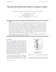
<strong>Particle</strong>-<strong>Based</strong> <strong>Fluid</strong> <strong>Simulation</strong> <strong>for</strong> <strong>Interactive</strong> Applications<br />
Matthias Müller, David Charypar and Markus Gross<br />
Department of Computer Science, Federal Institute of Technology Zürich (ETHZ), Switzerland<br />
Abstract<br />
Realistically animated fluids can add substantial realism to interactive applications such as virtual surgery simulators<br />
or computer games. In this paper we propose an interactive method based on Smoothed <strong>Particle</strong> Hydrodynamics<br />
(SPH) to simulate fluids with free surfaces. The method is an extension of the SPH-based technique<br />
by Desbrun to animate highly de<strong>for</strong>mable bodies. We gear the method towards fluid simulation by deriving the<br />
<strong>for</strong>ce density fields directly from the Navier-Stokes equation and by adding a term to model surface tension effects.<br />
In contrast to Eulerian grid-based approaches, the particle-based approach makes mass conservation equations<br />
and convection terms dispensable which reduces the complexity of the simulation. In addition, the particles can<br />
directly be used to render the surface of the fluid. We propose methods to track and visualize the free surface using<br />
point splatting and marching cubes-based surface reconstruction. Our animation method is fast enough to be used<br />
in interactive systems and to allow <strong>for</strong> user interaction with models consisting of up to 5000 particles.<br />
Categories and Subject Descriptors (according to ACM CCS): I.3.7 [Computer Graphics]: Three-Dimensional<br />
Graphics and Realism<br />
1. Introduction<br />
1.1. Motivation<br />
<strong>Fluid</strong>s (i.e. liquids and gases) play an important role in every<br />
day life. Examples <strong>for</strong> fluid phenomena are wind, weather,<br />
ocean waves, waves induced by ships or simply pouring of<br />
a glass of water. As simple and ordinary these phenomena<br />
may seem, as complex and difficult it is to simulate them.<br />
Even though Computational <strong>Fluid</strong> Dynamics (CFD) is a well<br />
established research area with a long history, there are still<br />
many open research problems in the field. The reason <strong>for</strong><br />
the complexity of fluid behavior is the complex interplay of<br />
various phenomena such as convection, diffusion, turbulence<br />
and surface tension. <strong>Fluid</strong> phenomena are typically simulated<br />
off-line and then visualized in a second step e.g. in<br />
aerodynamics or optimization of turbines or pipes with the<br />
goal of being as accurate as possible.<br />
Less accurate methods that allow the simulation of fluid<br />
effects in real-time open up a variety of new applications.<br />
In the fields mentioned above real-time methods help to<br />
test whether a certain concept is promising during the design<br />
phase. Other applications <strong>for</strong> real-time simulation tech-<br />
Figure 1: Pouring water into a glass at 5 frames per second.<br />
niques <strong>for</strong> fluids are medical simulators, computer games or<br />
any type of virtual environment.<br />
1.2. Related Work<br />
Computational <strong>Fluid</strong> Dynamics has a long history. In 1822<br />
Claude Navier and in 1845 George Stokes <strong>for</strong>mulated the<br />
famous Navier-Stokes Equations that describe the dynamics<br />
of fluids. Besides the Navier-Stokes equation which describes<br />
conservation of momentum, two additional equations<br />
namely a continuity equation describing mass conservation<br />
and a state equation describing energy conservac○<br />
The Eurographics Association 2003.
Müller et al / <strong>Particle</strong>-<strong>Based</strong> <strong>Fluid</strong> <strong>Simulation</strong> <strong>for</strong> <strong>Interactive</strong> Applications<br />
tion are needed to simulate fluids. Since those equations are<br />
known and computers are available to solve them numerically,<br />
a large number of methods have been proposed in the<br />
CFD literature to simulate fluids on computers.<br />
Since about two decades, special purpose fluid simulation<br />
techniques have been developed in the field of computer<br />
graphics. In 1983 T. Reeves 17 introduced particle systems as<br />
a technique <strong>for</strong> modeling a class of fuzzy objects. Since then<br />
both, the particle-based Lagrangian approach and the gridbased<br />
Eulerian approach have been used to simulate fluids<br />
in computer graphics. Desbrun and Cani 2 and Tonnesen 22<br />
use particles to animate soft objects. <strong>Particle</strong>s have also been<br />
used to animate surfaces 7 , to control implicit surfaces 23 and<br />
to animate lava flows 20 . In recent years the Eulerian approach<br />
has been more popular as <strong>for</strong> the simulation of fluids<br />
in general 18 , water 4, 3, 21 , soft objects 14 and melting effects 1 .<br />
So far only a few techniques optimized <strong>for</strong> the use in interactive<br />
systems are available. Stam’s method 18 that is grid<br />
based is certainly an important step towards real-time simulation<br />
of fluids. For the special case of fluids that can be represented<br />
by height fields, interactive animation techniques<br />
are available as well 6 .<br />
Here we propose a particle-based approach based on<br />
Smoothed <strong>Particle</strong> Hydrodynamics to animate arbitrary fluid<br />
motion.<br />
1.3. Our Contribution<br />
We propose a method based on Smoothed <strong>Particle</strong>s Hydrodynamics<br />
(SPH) 9 to simulate fluids with free surfaces. Stam<br />
and Fiume first introduced SPH to the graphics community<br />
to depict fire and other gaseous phenomena 19 . Later, Desbrun<br />
used SPH to animate highly de<strong>for</strong>mable bodies 2 .We<br />
extend his method focussing on the simulation of fluids. To<br />
this end, we derive the viscosity and pressure <strong>for</strong>ce fields directly<br />
from the Navier-Stokes equation and propose a way<br />
to model surface tension <strong>for</strong>ces. For the purpose of interactivity,<br />
we designed new special purpose smoothing kernels.<br />
Surface tracking and surface rendering at interactive rates<br />
are difficult problems <strong>for</strong> which we describe possible solutions.<br />
2. Smoothed <strong>Particle</strong> Hydrodynamics<br />
Although Smoothed <strong>Particle</strong> Hydrodynamics (SPH) was developed<br />
by Lucy 9 and Gingold and by Monaghan 5 <strong>for</strong> the<br />
simulation of astrophysical problems, the method is general<br />
enough to be used in any kind of fluid simulation. For introductions<br />
to SPH we refer the reader to Monaghan 10 or<br />
Münzel 13 .<br />
SPH is an interpolation method <strong>for</strong> particle systems. With<br />
SPH, field quantities that are only defined at discrete particle<br />
locations can be evaluated anywhere in space. For this<br />
purpose, SPH distributes quantities in a local neighborhood<br />
of each particle using radial symmetrical smoothing kernels.<br />
According to SPH, a scalar quantity A is interpolated at location<br />
r by a weighted sum of contributions from all particles:<br />
A j<br />
A S (r)=∑m j W(r − r j ,h), (1)<br />
j ρ j<br />
where j iterates over all particles, m j is the mass of particle<br />
j, r j its position, ρ j the density and A j the field quantity at<br />
r j .<br />
The function W(r,h) is called the smoothing kernel with<br />
core radius h. Since we only use kernels with finite support,<br />
we use h as the radius of support in our <strong>for</strong>mulation. If W is<br />
even (i.e. W(r,h)=W(−r,h)) and normalized, the interpolation<br />
is of second order accuracy. The kernel is normalized<br />
if<br />
∫<br />
W(r)dr = 1. (2)<br />
The particle mass and density appear in Eqn. (1) because<br />
each particle i represents a certain volume V i = m i /ρ i . While<br />
the mass m i is constant throughout the simulation and, in our<br />
case, the same <strong>for</strong> all the particles, the density ρ i varies and<br />
needs to be evaluated at every time step. Through substitution<br />
into Eqn. (1) we get <strong>for</strong> the density at location r:<br />
ρ j<br />
ρ S (r)=∑m j W(r − r j<br />
j ρ j<br />
,h)=∑m j W(r − r j ,h). (3)<br />
j<br />
In most fluid equations, derivatives of field quantities appear<br />
and need to be evaluated. With the SPH approach, such<br />
derivatives only affect the smoothing kernel. The gradient of<br />
A is simply<br />
A j<br />
∇A S (r)=∑m j ∇W(r − r j ,h) (4)<br />
j ρ j<br />
while the Laplacian of A evaluates to<br />
∇ 2 A j<br />
A S (r)=∑m j ∇ 2 W(r − r j ,h). (5)<br />
j ρ j<br />
It is important to realize that SPH holds some inherent problems.<br />
When using SPH to derive fluid equations <strong>for</strong> particles,<br />
these equations are not guaranteed to satisfy certain physical<br />
principals such as symmetry of <strong>for</strong>ces and conservation<br />
of momentum. The next section describes our SPH-based<br />
model and techniques to solve these SPH-related problems.<br />
3. Modelling <strong>Fluid</strong>s with <strong>Particle</strong>s<br />
In the Eulerian (grid based) <strong>for</strong>mulation, isothermal fluids<br />
are described by a velocity field v, a density field ρ and a<br />
pressure field p. The evolution of these quantities over time<br />
is given by two equations. The first equation assures conservation<br />
of mass<br />
∂ρ<br />
+ ∇·(ρv)=0, (6)<br />
∂t<br />
c○ The Eurographics Association 2003.
Müller et al / <strong>Particle</strong>-<strong>Based</strong> <strong>Fluid</strong> <strong>Simulation</strong> <strong>for</strong> <strong>Interactive</strong> Applications<br />
while the Navier-Stokes equation 15 <strong>for</strong>mulates conservation<br />
of momentum<br />
( )<br />
∂v<br />
ρ<br />
∂t + v ·∇v = −∇p + ρg + µ∇ 2 v, (7)<br />
where g is an external <strong>for</strong>ce density field and µ the viscosity<br />
of the fluid. Many <strong>for</strong>ms of the Navier-Stokes equation appear<br />
in the literature. Eqn. (7) represents a simplified version<br />
<strong>for</strong> incompressible fluids.<br />
The use of particles instead of a stationary grid simplifies<br />
these two equations substantially. First, because the number<br />
of particles is constant and each particle has a constant mass,<br />
mass conservation is guaranteed and Eqn. (6) can be omitted<br />
completely. Second, the expression ∂v/∂t +v·∇v on the<br />
left hand side of Eqn. (7) can be replaced by the substantial<br />
derivative Dv/Dt. Since the particles move with the fluid,<br />
the substantial derivative of the velocity field is simply the<br />
time derivative of the velocity of the particles meaning that<br />
the convective term v·∇v is not needed <strong>for</strong> particle systems.<br />
There are three <strong>for</strong>ce density fields left on the right hand<br />
side of Eqn. (7) modeling pressure (−∇p), external <strong>for</strong>ces<br />
(ρg) and viscosity (µ∇ 2 v). The sum of these <strong>for</strong>ce density<br />
fields f = −∇p + ρg + µ∇ 2 v determines the change of momentum<br />
ρ Dv<br />
Dt of the particles on the left hand side. For the<br />
acceleration of particle i we, thus, get:<br />
a i = dv i<br />
dt<br />
= f i<br />
ρ i<br />
, (8)<br />
where v i is the velocity of particle i and f i and ρ i are the <strong>for</strong>ce<br />
density field and the density field evaluated at the location of<br />
particle i, repectively. We will now describe how we model<br />
the <strong>for</strong>ce density terms using SPH.<br />
3.1. Pressure<br />
Application of the SPH rule described in Eqn. (1) to the pressure<br />
term −∇p yields<br />
f pressure<br />
i<br />
p j<br />
= −∇p(r i )=−∑m j ∇W(r i − r j ,h). (9)<br />
j ρ j<br />
Un<strong>for</strong>tunately, this <strong>for</strong>ce is not symmetric as can be seen<br />
when only two particles interact. Since the gradient of the<br />
kernel is zero at its center, particle i only uses the pressure of<br />
particle j to compute its pressure <strong>for</strong>ce and vice versa. Because<br />
the pressures at the locations of the two particles are<br />
not equal in general, the pressure <strong>for</strong>ces will not be symmetric.<br />
Different ways of symmetrization of Eqn. (9) have been<br />
proposed in the literature. We suggest a very simple solution<br />
which we found to be best suited <strong>for</strong> our purposes of speed<br />
and stability<br />
f pressure<br />
i<br />
p i + p j<br />
= −∑m j ∇W(r i − r j ,h).. (10)<br />
j 2ρ j<br />
The so computed pressure <strong>for</strong>ce is symmetric because it uses<br />
the arithmetic mean of the pressures of interacting particles.<br />
Since particles only carry the three quantities mass, position<br />
and velocity, the pressure at particle locations has to be<br />
evaluated first. This is done in two steps. Eqn. (3) yields the<br />
density at the location of the particle. Then, the pressure can<br />
be computed via the ideal gas state equation<br />
p = kρ, (11)<br />
where k is a gas constant that depends on the temperature.<br />
In our simulations we use a modified version of Eqn. (11)<br />
suggested by Desbrun 2 p = k(ρ − ρ 0 ), (12)<br />
where ρ 0 is the rest density. Since pressure <strong>for</strong>ces depend on<br />
the gradient of the pressure field, the offset mathematically<br />
has not effect on pressure <strong>for</strong>ces. However, the offset does<br />
influence the gradient of a field smoothed by SPH and makes<br />
the simulation numerically more stable.<br />
3.2. Viscosity<br />
Application of the SPH rule to the viscosity term µ∇ 2 v again<br />
yields asymmetric <strong>for</strong>ces<br />
f viscosity<br />
i<br />
= µ∇ 2 v j<br />
v(r a)=µ∑m j ∇ 2 W(r i − r j ,h). (13)<br />
j ρ j<br />
because the velocity field varies from particle to particle.<br />
Since viscosity <strong>for</strong>ces are only dependent on velocity differences<br />
and not on absolute velocities, there is a natural way<br />
to symmetrize the viscosity <strong>for</strong>ces by using velocity differences:<br />
f viscosity<br />
i = µ∑<br />
j<br />
m j<br />
v j − v i<br />
ρ j<br />
∇ 2 W(r i − r j ,h). (14)<br />
A possible interpretation of Eqn. (14) is to look at the neighbors<br />
of particle i from i’s own moving frame of reference.<br />
Then particle i is accelerated in the direction of the relative<br />
speed of its environment.<br />
3.3. Surface Tension<br />
We model surface tension <strong>for</strong>ces (not present in Eqn. (7))<br />
explicitly based on ideas of Morris 12 . Molecules in a fluid<br />
are subject to attractive <strong>for</strong>ces from neighboring molecules.<br />
Inside the fluid these intermolecular <strong>for</strong>ces are equal in all<br />
directions and balance each other. In contrast, the <strong>for</strong>ces acting<br />
on molecules at the free surface are unbalanced. The net<br />
<strong>for</strong>ces (i.e. surface tension <strong>for</strong>ces) act in the direction of the<br />
surface normal towards the fluid. They also tend to minimize<br />
the curvature of the surface. The larger the curvature,<br />
the higher the <strong>for</strong>ce. Surface tension also depends on a tension<br />
coefficient σ which depends on the two fluids that <strong>for</strong>m<br />
the surface.<br />
The surface of the fluid can be found by using an additional<br />
field quantity which is 1 at particle locations and 0<br />
c○ The Eurographics Association 2003.
Müller et al / <strong>Particle</strong>-<strong>Based</strong> <strong>Fluid</strong> <strong>Simulation</strong> <strong>for</strong> <strong>Interactive</strong> Applications<br />
everywhere else. This field is called color field in the literature.<br />
For the smoothed color field we get:<br />
1<br />
c S (r)=∑m j W(r − r j ,h). (15)<br />
j ρ j<br />
The gradient field of the smoothed color field<br />
n = ∇c s (16)<br />
yields the surface normal field pointing into the fluid and the<br />
divergence of n measures the curvature of the surface<br />
κ = −∇2 c s<br />
. (17)<br />
|n|<br />
The minus is necessary to get positive curvature <strong>for</strong> convex<br />
fluid volumes. Putting it all together, we get <strong>for</strong> the surface<br />
traction:<br />
t surface = σκ n<br />
(18)<br />
|n|<br />
To distribute the surface traction among particles near the<br />
surface and to get a <strong>for</strong>ce density we multiply by a normalized<br />
scalar field δ s = |n| which is non-zero only near the<br />
surface. For the <strong>for</strong>ce density acting near the surface we get<br />
f surface = σκn = −σ∇ 2 n<br />
c S (19)<br />
|n|<br />
Evaluating n/|n| at locations where |n| is small causes numerical<br />
problems. We only evaluate the <strong>for</strong>ce if |n| exceeds<br />
a certain threshold.<br />
3.4. External Forces<br />
Our simulator supports external <strong>for</strong>ces such as gravity, collision<br />
<strong>for</strong>ces and <strong>for</strong>ces caused by user interaction. These<br />
<strong>for</strong>ces are applied directly to the particles without the use of<br />
SPH. When particles collide with solid objects such as the<br />
glass in our examples, we simply push them out of the object<br />
and reflect the velocity component that is perpendicular<br />
to the object’s surface.<br />
3.5. Smoothing Kernels<br />
Stability, accuracy and speed of the SPH method highly depend<br />
on the choice of the smoothing kernels. The kernels<br />
we use have second order interpolation errors because they<br />
are all even and normalized (see Fig. 2). In addition, kernels<br />
that are zero with vanishing derivatives at the boundary are<br />
conducive to stability. Apart from those constraints, one is<br />
free to design kernels <strong>for</strong> special purposes. We designed the<br />
following kernel<br />
{<br />
W poly6 (r,h)= 315 (h 2 − r 2 ) 3 0 ≤ r ≤ h<br />
64πh 9 (20)<br />
0 otherwise<br />
and use it in all but two cases. An important feature of this<br />
simple kernel is that r only appears squared which means<br />
2<br />
1<br />
–1 –0.8 –0.6 –0.4 –0.2 0 0.2 0.4 0.6 0.8 1<br />
–1<br />
–2<br />
14<br />
12<br />
10<br />
8<br />
6<br />
4<br />
2<br />
–1 –0.8 –0.6 –0.4 –0.2 0 0.2 0.4 0.6 0.8 1<br />
–2<br />
2<br />
1.8<br />
1.6<br />
1.4<br />
1.2<br />
0.8<br />
0.6<br />
0.4<br />
1<br />
0.2<br />
–1 –0.8 –0.6 –0.4 –0.2 0 0.2 0.4 0.6 0.8 1<br />
Figure 2: The three smoothing kernels W poly6 ,W spiky and<br />
W viscosity (from left to right) we use in our simulations. The<br />
thick lines show the kernels, the thin lines their gradients<br />
in the direction towards the center and the dashed lines the<br />
Laplacian. Note that the diagrams are differently scaled. The<br />
curves show 3-d kernels along one axis through the center<br />
<strong>for</strong> smoothing length h = 1.<br />
that is can be evaluated without computing square roots in<br />
distance computations. However, if this kernel is used <strong>for</strong> the<br />
computation of the pressure <strong>for</strong>ces, particles tend to build<br />
clusters under high pressure. As particles get very close to<br />
each other, the repulsion <strong>for</strong>ce vanishes because the gradient<br />
of the kernel approaches zero at the center. Desbrun 2 solves<br />
this problem by using a spiky kernel with a non vanishing<br />
gradient near the center. For pressure computations we use<br />
Debrun’s spiky kernel<br />
{<br />
W spiky (r,h)= 15 (h − r) 3 0 ≤ r ≤ h<br />
πh 6 0 otherwise,<br />
(21)<br />
that generates the necessary repulsion <strong>for</strong>ces. At the boundary<br />
where it vanishes it also has zero first and second derivatives.<br />
Viscosity is a phenomenon that is caused by friction and,<br />
thus, decreases the fluid’s kinetic energy by converting it into<br />
heat. There<strong>for</strong>e, viscosity should only have a smoothing effect<br />
on the velocity field. However, if a standard kernel is<br />
used <strong>for</strong> viscosity, the resulting viscosity <strong>for</strong>ces do not always<br />
have this property. For two particles that get close to<br />
each other, the Laplacian of the smoothed velocity field (on<br />
which viscosity <strong>for</strong>ces depend) can get negative resulting in<br />
<strong>for</strong>ces that increase their relative velocity. The artifact appears<br />
in coarsely sampled velocity fields. In real-time applications<br />
where the number of particles is relatively low, this<br />
effect can cause stability problems. For the computation of<br />
viscosity <strong>for</strong>ces we, thus, designed a third kernel:<br />
{<br />
W viscosity (r,h)= 15 − r3 + r2 + h<br />
2πh 3 2h 3 h 2 2r − 1 0≤ r ≤ h<br />
0 otherwise.<br />
(22)<br />
whose Laplacian is positive everywhere with the following<br />
c○ The Eurographics Association 2003.
Müller et al / <strong>Particle</strong>-<strong>Based</strong> <strong>Fluid</strong> <strong>Simulation</strong> <strong>for</strong> <strong>Interactive</strong> Applications<br />
additional properties:<br />
∇ 2 W(r,h) = 45 (h − r)<br />
πh6 W(|r| = h,h) = 0<br />
∇W(|r| = h,h) = 0<br />
The use of this kernel <strong>for</strong> viscosity computations increased<br />
the stability of the simulation significantly allowing to omit<br />
any kind of additional damping.<br />
3.6. <strong>Simulation</strong><br />
For the integration of the Eqn. (8) we use the Leap-Frog<br />
scheme 16 . As a second order scheme <strong>for</strong> which the <strong>for</strong>ces<br />
need to be evaluation only once, it best fits our purposes and<br />
in our examples allows time steps up to 10 milliseconds. For<br />
the examples we used constant time steps. We expect even<br />
better per<strong>for</strong>mance if adaptive time steps are used based on<br />
the Courant-Friedrichs-Lewy condition 2 .<br />
4. Surface Tracking and Visualization<br />
The color field c S and its gradient field n = ∇c S defined in<br />
section 3.3 can be used to identify surface particles and to<br />
compute surface normals. We identify a particle i as a surface<br />
particle if<br />
|n(r i )| > l, (23)<br />
where l is a threshold parameter. The direction of the surface<br />
normal at the location of particle i is given by<br />
−n(r i ). (24)<br />
4.1. Point Splatting<br />
We now have a set of points with normals but without<br />
connectivity in<strong>for</strong>mation. This is exactly the type of in<strong>for</strong>mation<br />
needed <strong>for</strong> point splatting techniques 24 . However,<br />
these methods are designed to work with point clouds obtained<br />
from scanners that typically contain at least 10,000<br />
to 100,000 points. We only use a few thousand particles a<br />
fraction of which are identified as being on the surface. Still<br />
surface splatting yields plausible results as shown in the results<br />
section.<br />
We are currently working on ways to upsample the surface<br />
of the fluid. Hereby, the color field in<strong>for</strong>mation of surface<br />
particles is interpolated to find locations <strong>for</strong> additional<br />
particles on the surface only used <strong>for</strong> rendering.<br />
4.2. Marching Cubes<br />
Another way to visualize the free surface is by rendering an<br />
iso surface of the color field c S . We use the marching cubes<br />
algorithm 8 to triangulate the iso surface. In a grid fixed in<br />
space the cells that contain the surface are first identified.<br />
We start searches from all the cells that contain surface particles<br />
and from there recursively traverse the grid along the<br />
surface. With the use of a hash table we make sure that the<br />
cells are not visited more than once. For each cell identified<br />
to contain the surface, the triangles are generated via a fast<br />
table lookup.<br />
5. Implementation<br />
Since the smoothing kernels used in SPH have finite support<br />
h, a common way to reduce the computational complexity is<br />
to use a grid of cells of size h. Then potentially interacting<br />
partners of a particle i only need to be searched in i’s own<br />
cell and all the neighboring cells. This technique reduces the<br />
time complexity of the <strong>for</strong>ce computation step from O(n 2 )<br />
to O(nm), m being the average number of particles per grid<br />
cell.<br />
With a simple additional trick we were able to speed<br />
up the simulation by an additional factor of 10. Instead of<br />
storing references to particles in the grid, we store copies<br />
of the particle objects in the grid cells (doubling memory<br />
consumption). The reason <strong>for</strong> the speed up is the proximity<br />
in memory of the in<strong>for</strong>mation needed <strong>for</strong> interpolation<br />
which dramatically increases the cash hit rate. Further<br />
speedup might be possible through even better clustering using<br />
Hilbert space filling curves 11 . The data structure <strong>for</strong> fast<br />
neighbor searches is also used <strong>for</strong> surface tracking and rendering.<br />
6. Results<br />
The water in the glass shown in Fig. 3 is sampled with 2200<br />
particles. An external rotational <strong>for</strong>ce field causes the fluid<br />
to swirl. The first image (a) shows the individual particles.<br />
For the second image (b), point splatting was used to render<br />
the free surface only. In both modes, the animation runs<br />
at 20 frames per second on a 1.8 GHz Pentium IV PC with<br />
a GForce 4 graphics card. The most convincing results are<br />
produced when the iso surface of the color field is visualized<br />
using the marching cubes algorithm as in image (c).<br />
However, in this mode the frame rate drops to 5 frames per<br />
second. Still this frame rate is significantly higher than the<br />
one of most off-line fluid simulation techniques and with the<br />
next generation of graphics hardware, real-time per<strong>for</strong>mance<br />
will be possible.<br />
The image sequence shown in Fig. 4 demonstrates interaction<br />
with the fluid. Through mouse motion, the user generates<br />
an external <strong>for</strong>ce field that cause the water to splash.<br />
The free surface is rendered using point splatting while isolated<br />
particles are drawn as single droplets. The simulation<br />
with 1300 particles runs at 25 frames per second.<br />
For the animation shown in Fig. 5 we used 3000 particles<br />
and rendered the surface with the marching cubes technique<br />
at 5 frames per second.<br />
c○ The Eurographics Association 2003.
Müller et al / <strong>Particle</strong>-<strong>Based</strong> <strong>Fluid</strong> <strong>Simulation</strong> <strong>for</strong> <strong>Interactive</strong> Applications<br />
7. Conclusions and Future Work<br />
We have presented a particle-based method <strong>for</strong> interactive<br />
fluid simulation and rendering. The physical model is based<br />
on Smoothed <strong>Particle</strong> Hydrodynamics and uses special purpose<br />
kernels to increase stability and speed. We have presented<br />
techniques to track and render the free surface of fluids.<br />
The results are not as photorealistic yet as animations<br />
computed off-line. However, given that the simulation runs<br />
at interactive rates instead of taking minutes or hours per<br />
frame as in today’s off-line methods, the results are quite<br />
promising.<br />
While we are quite content with the physical model, tracking<br />
and rendering of the fluid surface in real time certainly<br />
remains an open research problem. In the future we will investigate<br />
upsampling techniques as well as ways to increase<br />
the per<strong>for</strong>mance of the marching cubes-based algorithm.<br />
Acknowledgements<br />
The authors would like to thank Simone Hieber <strong>for</strong> her helpful<br />
comments and Rolf Bruderer, Simon Schirm and Thomas<br />
Rusterholz <strong>for</strong> their contributions to the real-time system.<br />
References<br />
1. Mark Carlson, Peter J. Mucha, III R. Brooks Van Horn, and<br />
Greg Turk. Melting and flowing. In Proceedings of the ACM<br />
SIGGRAPH symposium on Computer animation, pages 167–<br />
174. ACM Press, 2002.<br />
2. M. Desbrun and M. P. Cani. Smoothed particles: A new<br />
paradigm <strong>for</strong> animating highly de<strong>for</strong>mable bodies. In<br />
Computer Animation and <strong>Simulation</strong> ’96 (Proceedings of<br />
EG Workshop on Animation and <strong>Simulation</strong>), pages 61–76.<br />
Springer-Verlag, Aug 1996.<br />
3. D. Enright, S. Marschner, and R. Fedkiw. Animation and rendering<br />
of complex water surfaces. In Proceedings of the 29th<br />
annual conference on Computer graphics and interactive techniques,<br />
pages 736–744. ACM Press, 2002.<br />
4. N. Foster and R. Fedkiw. Practical animation of liquids.<br />
In Proceedings of the 28th annual conference on Computer<br />
graphics and interactive techniques, pages 23–30. ACM Press,<br />
2001.<br />
5. R. A. Gingold and J. J. Monaghan. Smoothed particle hydrodynamics:<br />
theory and application to non-spherical stars.<br />
Monthly Notices of the Royal Astronomical Society, 181:375–<br />
398, 1977.<br />
6. Damien Hinsinger, Fabrice Neyret, and Marie-Paule Cani. <strong>Interactive</strong><br />
animation of ocean waves. In Proceedings of the<br />
ACM SIGGRAPH symposium on Computer animation, pages<br />
161–166. ACM Press, 2002.<br />
7. Jean-Christophe Lombardo and Claude Puech. Oriented particles:<br />
A tool <strong>for</strong> shape memory objects modelling. In Graphics<br />
Interface’95, pages 255–262, mai 1995. Quebec city, Canada.<br />
8. William E. Lorensen and Harvey E. Cline. Marching cubes:<br />
A high resolution 3d surface construction algorithm. In Proceedings<br />
of the 14th annual conference on Computer graphics<br />
and interactive techniques, pages 163–169. ACM Press, 1987.<br />
9. L. B. Lucy. A numerical approach to the testing of the fission<br />
hypothesis. The Astronomical Journal, 82:1013–1024, 1977.<br />
10. J. J. Monaghan. Smoothed particle hydrodynamics. Annual<br />
Review of Astronomy and Astrophysics, 30:543–574, 1992.<br />
11. B. Moon, H. V. Jagadish, C. Faloutsos, and J. H. Saltz. Analysis<br />
of the clustering properties of hilbert space-filling curve.<br />
IEEE Transactions on Knowledge and Data Engineering,<br />
13(1):124–141, 2001.<br />
12. J. P. Morris. Simulating surface tension with smoothed particle<br />
hydrodynamics. International Journal <strong>for</strong> Numerical Methods<br />
in <strong>Fluid</strong>s, 33(3):333–353, 2000.<br />
13. S. A. Münzel. Smoothed <strong>Particle</strong> Hydrodynamics und ihre Anwendung<br />
auf Akkretionsscheiben. PhD thesis, Eberhard-Karls-<br />
Universität Thübingen, 1996.<br />
14. D. Nixon and R. Lobb. A fluid-based soft-object model.<br />
IEEE Computer Graphics and Applications, pages 68–75,<br />
July/August 2002.<br />
15. D. Pnueli and C. Gutfinger. <strong>Fluid</strong> Mechanics. Cambridge<br />
Univ. Press, NY, 1992.<br />
16. C. Pozrikidis. Numerical Computation in Science and Engineering.<br />
Ox<strong>for</strong>d Univ. Press, NY, 1998.<br />
17. W. T. Reeves. <strong>Particle</strong> systems — a technique <strong>for</strong> modeling a<br />
class of fuzzy objects. ACM Transactions on Graphics 2(2),<br />
pages 91–108, 1983.<br />
18. Jos Stam. Stable fluids. In Proceedings of the 26th annual<br />
conference on Computer graphics and interactive techniques,<br />
pages 121–128. ACM Press/Addison-Wesley Publishing Co.,<br />
1999.<br />
19. Jos Stam and Eugene Fiume. Depicting fire and other gaseous<br />
phenomena using diffusion processes. Computer Graphics,<br />
29(Annual Conference Series):129–136, 1995.<br />
20. Dan Stora, Pierre-Olivier Agliati, Marie-Paule Cani, Fabrice<br />
Neyret, and Jean-Dominique Gascuel. Animating lava flows.<br />
In Graphics Interface, pages 203–210, 1999.<br />
21. T. Takahashi, U. Heihachi, A. Kunimatsu, and H. Fujii. The<br />
simulation of fluid-rigid body interaction. ACM Siggraph<br />
Sketches & Applications, July 2002.<br />
22. D. Tonnesen. Dynamically Coupled <strong>Particle</strong> Systems <strong>for</strong> Geometric<br />
Modeling, Reconstruction, and Animation. PhD thesis,<br />
University of Toronto, November 1998.<br />
23. Andrew Witkin and Paul Heckbert. Using particles to sample<br />
and control implicit surfaces. In Computer Graphics (Proc.<br />
SIGGRAPH ’94), volume 28, 1994.<br />
24. Matthias Zwicker, Hanspeter Pfister, Jeroen van Baar, and<br />
Markus Gross. Surface splatting. In Proceedings of the 28th<br />
annual conference on Computer graphics and interactive techniques,<br />
pages 371–378. ACM Press, 2001.<br />
c○ The Eurographics Association 2003.
Müller et al / <strong>Particle</strong>-<strong>Based</strong> <strong>Fluid</strong> <strong>Simulation</strong> <strong>for</strong> <strong>Interactive</strong> Applications<br />
(a) (b) (c)<br />
Figure 3: A swirl in a glass induced by a rotational <strong>for</strong>ce field. Image (a) shows the particles, (b) the surface using point<br />
splatting and (c) the iso-surface triangulated via marching cubes.<br />
Figure 4: The user interacts with the fluid causing it to splash.<br />
Figure 5: Pouring water into a glass at 5 frames per second.<br />
c○ The Eurographics Association 2003.