Computational Vision U. Minn. Psy 5036 Daniel Kersten Lecture 6

Computational Vision 

U. Minn. Psy 5036 

Daniel Kersten 

Lecture 6 

http://vision.psych.umn.edu/www/kersten-lab/courses/Psy5036/SyllabusF2000.html) 

‡ Initialize standard library files: 

6.ProbabilityPatternIIb.nb 3 

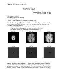
Illumination 

h = 

1 

Face 

s i = 

2 

One example is in shape from shading. An image provides the "test measurements" that can be used to estimate an object's 

shape and/or estimate the direction of illumination. Accurate object identification often depends crucially on an object's 

shape, and the illumination is a confounding (secondary) variable. This suggests that visual recognition should put a high 

cost to errors in shape perception, and lower costs on errors in illumination direction estimation. So the process of perceptual 

inference depends an task. The effect of marginalization in the fruit example illustrated task-dependence. Now we 

show how marginalization can be generalized through decision theory to model other kinds of goals than error minimization 

(MAP) in task-dependence. 

Bayes Decision theory provides the means to model visual performance as a function of utility. 

Some terminology. We've used the terms switch state, hypothesis, signal state as essentially the same--to represent the 

random variable indicating the state of the world--the "state space". So far, we've assumed that the decision, d, of the 

observer maps directly to state space, d->s. We now clearly distinguish the decision space from the state or hypothesis 

space, and introduce the idea of a loss L(d,s), which is the cost for making the decision d, when the actual state is s. 

Often we can't directly measure s, and we can only infer it from observations. Thus, given an observation (image measurement) 

x, we define a risk function that represents the average loss over signal states s: 

R Hd; xL = ‚ 

s 

L Hd, sL p Hs » xL 

(1) 

This suggests a decision rule: a(x)=argmin R(d;x). But not all x are equally likely. This decision rule minimizes the 

expected risk average over all observations: 

d 

R HaL = ‚ 

s 

R Hd; xL p HxL 

(2) 

We won't show them all here, but with suitable choices of likelihood, prior, and loss functions, we can derive standard 

estimation procedures (maximum likelihood, MAP, estimation of the mean) as special cases. 

For the MAP estimator, 

R Hd; xL = ‚ L Hd, sL p Hs » xL = ‚ 

s 

s 

H1 -dd,sL p Hs » xL = 1 - p Hd » xL 

(3) 

where dd,sis the discrete analog to the Dirac delta function--it is zero if d≠s, and one if d=s. 

Thus minimizing risk with the loss function L = H1 -d d,s Lis equivalent to maximizing the posterior, p(d|x). 

What about marginalization? You can see from the definition of the risk function, that this corresponds to a uniform loss: 

L = -1. 

4 6.ProbabilityPatternIIb.nb 

R Hs1; xL = ‚ 

s2 

L Hd2, s2L p Hs1, s2 » xL 

(4) 

So for our face recognition example, a really huge error in illumination direction has the same cost as getting it right.For the 

fruit example, optimal classification of the fruit identity required marginalizing over fruit color--i.e. effectively treating fruit 

color identification errors as equally costly...even tho', doing MAP after marginalization effectively means we are not 

explicitly identifying color. 

Graphical models for Hypothesis Inference: Three types 

Three types of nodes in a graphical model: known, unknown to be estimated, unknown 

to be integrated out (marginalized) 

We have three basic states for nodes in a graphical model: known , unknown to be estimated, unknown to be integrated out 

(marginalization). We have causal state of the world S, that gets mapped to some image data I, through some intermediate 

parameters M: S->M->I. So face identity S determines facial shape M, which in turn determines the image I itself. Consider 

three very broad types of task: 

Image synthesis (forward, generative model): We want to model I through p(I|S). In our example, we want to specify 

"Bill", and then p(I|S="Bill") can be used implemented as an algorithm to spit out images of Bill. M gets integrated out. 

Hypothesis inference: we want to model samples for S : p(S|I). Given an image, we want to spit out likely object identities, 

so that we can minimize risk, or do MAP classification for accurate object identification. M gets integrated out again. 

Learning: we want to model M: p(M|I,S), to learn how the intermediate variables are distributed. Given lots of samples of 

objects and their images, we want to learn the mapping parameters between them. (Alternatively, do a mental switch and 

consider a neural network in which an input S gets mapped to an output I through intermediate variables M. We can think of 

M as representing synaptic weights to be learned.) 

Regression: estimating parameters that provide a good fit to data. E.g. slope and intercept for a straight line through points 

{xi,yi}. 

Density estimation: Regression on a probability density functions, with the added condition that the area under the fitted 

curve must sum to one. 

Hypothesis inference: Three types 

‡ Detection 

Let the decision variable d, be represented by s`.



‡ Classification 

MAP rule: argmax 

8pHSi » x


‡ Continous estimation 

argmax 

S 

8pHS » xP (S =sd |x ). This is 

exactly like the problem of guessing “heads ”or “tails ” for a biased coin, say with a probability of heads P (S =sb|x ). 

Imagine the light discrimination experiment repeated many times and you have to decide whether the switch was set to 

bright or not –but only on those trials for which you measured exactly x .The optimal strategy is to always say “bright ”. 

Let's see why. First note that: 

p(error|x) = p(say "bright", actually dim |x) + p(say "dim", actually bright |x) = 

p(s1` , s2 | x)+p(s1, s2` | x) 

Given x, the response is independent of the actual signal state (see graphical model for detection above--"response is 

conditionally independent of signal state, given observation x"), so the joint probabilities factor: 

p(error|x) = p(say "bright" |x)p(actually dim |x) + p(say "dim" |x)p(actually bright |x) 

Let t= p(say "bright" |x), then 

p(error|t,x) = t*p(actually dim |x) + (1-t)*p(actually bright |x).


p(error|t), as a function of t, defines a straight line with slope p(actually dim |x)-p(actually bright |x). (Just take the 

partial derivative with respect to t.) We've assumed P (S =sb |x )>P (S =s d |x )), so p(error|t) has a negative slope, with the 

smallest non-negative value of t being one. So, error is minimized when t=p(say "bright" |x)=1. I.e. Always say "bright". 

pHerror 

0.8 

0.7 

0.6 

0.5 

0.4 

0.3 

0.2 0.4 0.6 0.8 1 t 

Always saying "bright" results in a probability of error P (error |x )=P (S =sd |x ).That’s the best that can be done on average. 

On the other hand, if the observation is in a region for which P (S =sd|x )>P (S =sb |x ),the minimum error strategy is to 

always pick “dim” with a resulting P (error |x )=P (S =sb |x ).Of course, x isn’t fixed from trial to trial, so we calculate the 

total probability of error which is determined by the specific values where signal states and decisions don ’t agree: 

` 

p(error)=⁄ i∫j pHsi , s jL 

` 

=⁄ i∫j Ÿ pHsi , s j » xL pHxL „ 

` 

x=⁄ i∫j Ÿ pHsi » xL pHs j » xL pHxL „ x 

Because the MAP rule ensures that 

` 

pHsi , s j » xL is the minimum for each x, the integral over all x minimizes the total probability 

of error. 

Ideal pattern detector for a signal which is exactly known (SKE) 

In this notebook we will study an ideal detector called the signal-known-exactly ideal (SKE). This detector has a built-in 

template that matches the signal that it is looking for. The signal is embedded (by adding pixel intensity values) in "white 

gaussian noise". "white" means the pixels are not correlated with each other--intuitively this means that you can't reliably 

predict what one pixel's value is from any of the others. Assignment 1 simulates the behavior of this ideal. In the absence of 

any internal noise, this ideal detector behaves as one would expect a linear neuron to behave when a target signal pattern 

exactly matches its synaptic weight pattern. There are some neurons in the the primary cortex of the visual system called 

"simple cells". These cells can be modeled as ideal detectors for the patterns that match their receptive fields. In actual 

practice, neurons are not noise-free, and not perfectly linear. 


Calculating the Pattern Ideal's d' based on signal-to-noise ratio 

‡ Overview 

The generative model is a straightfoward extension of the single variable gaussian model, to patterns. s[i] represents the 

signal pattern values at pixel locations i=1..M: 

H = signal pattern: x[i] = s[i] + n[i], where n[i] ~ N(0,s), i.i.d. 

H = no signal pattern: x[i] = 0 + n[i], where n[i] ~ N(0,s), i.i.d. 

(i.i.d. is probability jargon meaning that the random variables are "independently drawn and identically distributed". N(m,s) 

means "normal distribution" or gaussian, with mean m and standard deviation s.) 

We are going to do two things: 

1. Prove that a simple decision variable for detecting a known fixed pattern in white gaussian noise is the dot product of the 

observation image with the known signal image: r = s.x 

2. Show that d' is given by: d'= m 2-m1 

ÅÅÅÅÅÅÅÅÅÅÅÅÅ 

sr 

= è!!!!! s.s 

ÅÅÅÅÅÅÅÅÅÅÅ 

s 

‡ 1. Proof that cross-correlation produces an ideal decision variable: 

Let r be the decision variable. By definition: 

d'= m 2-m1 

ÅÅÅÅÅÅÅÅÅÅÅÅÅÅ 

sr 

(5) 

where u2 is the mean of the decision variable, r, under the signal hypothesis, u1 is the mean under the noise-only hypothesis. 

sr is the standard deviation of r, assumed to be the same under both hypotheses (we'll show this to be true below). But 

what is the decision variable? Starting from the maximum a posteriori rule, we saw that basing decisions on the likelihood 

ratio is ideal, in particular we could minimize the probability of error with the appropriate decision criterion. So the likelihood 

ratio is a decision variable. But it isn't the only one, because any monotonic function is still optimal. So our goal is to 

pick a decision variable which is simple, intuitive, and easy to compute. 

First, we need an expression for the likelihood ratio: 

p Hx » signal plus noiseL 

ÅÅÅÅÅÅÅÅÅÅÅÅÅÅÅÅÅÅÅÅÅÅÅÅÅÅÅÅÅÅÅÅ ÅÅÅÅÅÅÅÅÅÅÅÅÅÅÅÅÅÅÅÅÅÅÅÅÅÅÅÅÅ 

p Hx » noise onlyL 

(6) 

where x is the vector representing the image measurements actually observed. For pixel i, 

x[i] = s[i] + n[i], under signal plus gaussian noise condition 

x[i] = n[i], under gaussian noise only condition 

(7) 

Consider just one pixel of intensity x. Under the signal plus noise condition, the values of x fluctuate about the average 

signal intensity s with a Gaussian distribution (gp[]) with mean s and standard deviation s. 

(Note that s[i] is the average value of a pixel intensity at location i. But m1 and m2 are the averages of the decision variable


r--our goal will be to calculate these in the following subsection on d') 

So under the signal plus noise condition, the likelihood p[x|signal] is the gp[x-s; s]: 

gp[x_,s_,s_]:= (1/(s*Sqrt[2 Pi])) Exp[-(x-s)^2/(2 s^2)] 

gp[x,s,s] 

‰ - ÅÅÅÅÅÅÅÅÅÅÅÅÅÅÅÅ H-s+xL2 ÅÅÅÅÅÅ 

2 s 

ÅÅÅÅÅÅÅÅÅÅÅÅÅÅÅÅ 

2 

è!!!!!!! 

2 ps 

ÅÅÅÅÅÅÅ 

Again, consider just one pixel of intensity x. Under the noise only condition, the values of x fluctuate about the average 

intensity corresponding to the mean of the noise, which we assume is zero. 

So under the noise only condition, the likelihood p[x|noise] is: 

gp[x,0,s] 

‰ - ÅÅÅÅÅÅÅÅ 

x2 ÅÅÅÅÅÅÅÅÅ 

2 s 2 

ÅÅÅÅÅÅÅÅÅÅÅÅÅÅÅÅ è!!!!!! 

2 p ÅÅÅÅÅÅÅ 

s 

But we actually have a whole pattern of values of x, which make up an image vector x. So consider a pattern of image 

intensities represented now by a vector x = {x[1],x[2],...x[N]}. Let the mean values of each pixel under the signal plus noise 

condition be given by vector s = {s[1],s[2],...,s[N]}. The joint probability of an image observation x, under the signal 

hypothesis is p(x|s): 

Product[gp[x[i],s[i],s],{i,1,N}] 

N 

Â 

i=1 

‰ - ÅÅÅÅÅÅÅÅÅÅÅÅÅÅÅÅ H-s@iD+x@iDL2 ÅÅÅÅÅÅÅÅÅÅÅÅÅÅÅÅÅÅÅÅÅÅ 

2 s2 

ÅÅÅÅÅÅÅÅÅÅÅÅÅÅÅÅ è!!!!!!! ÅÅÅÅÅÅÅÅÅÅÅÅÅÅÅÅÅ 

2 ps 

This is because we are assuming independence (whether we are right or not depends on the problem). But independence 

between pixels means we can multiply the individual probabilities to get the global joint image probability. 

The joint probability of an image observation x, under the noise only hypothesis is: 

Product[gp[x[i],0,s],{i,1,M}] 

N 

Â 

i=1 

‰ - ÅÅÅÅÅÅÅÅÅÅÅÅÅÅÅ 

x@iD2 

2 s2 

ÅÅÅÅÅÅÅÅÅÅÅÅÅÅÅÅÅ è!!!!!!! 

2 ps 


Now we have what we need for the likelihood ratio: 

Product@gp@x@iD, s@iD, sD, 8i, 1, M


s@1D x@1D + s@2D x@2D 

(8) 

But this is just the dot product of the image x with the signal s. 

So in general, to recap using full summation notation, the log likelihood ratio is: 

log 

i 

M 

j Â k i=1 

‰ - ÅÅÅÅÅÅÅÅÅÅÅÅÅÅÅÅÅÅÅÅÅÅÅÅÅÅÅÅÅÅÅÅ 

Hx HiL-s HiLL2 ÅÅÅÅÅÅÅÅÅÅÅÅÅÅÅÅ -Hx ÅÅÅÅÅÅÅÅÅÅÅÅÅÅÅÅ HiLL 2 

2 s 

ÅÅÅÅÅÅÅÅÅÅÅÅÅÅÅÅÅÅÅÅÅÅÅÅÅÅÅÅÅÅÅÅ 

2 

è!!!!!!! ÅÅÅÅÅÅÅÅÅÅÅÅÅÅÅÅÅÅ 

2 ps 

y 

z 

{ 

(9) 

which is monotonic with: 

M 

LogA‰ 

i=1 

‰ 

M 

2 xHiL sHiL 

ÅÅÅÅÅÅÅÅÅÅÅÅÅÅÅÅ ÅÅÅÅÅÅÅÅÅÅÅÅ 

2 s2 

E = H1 ê s 2 L ‚ 

i=1 

xHiL sHiL 

(10) 

which is monotonic with: 

M 

r = ‚ 

i=1 

xHiL sHiL = Sum@x@iD s@iD, 8i, 1,N


Psychophysical tasks & techniques 

The Receiver Operating Characteristic (ROC) 

Although we can't directly measure the internal distributions of a human observer's decision variable, we've seen that we 

can measure hit and false alarm rates, and thus d'. But one can do more, and actually test to see if an observer's decisions are 

consistent with Gaussian distributions with equal variance. If the criterion is varied, we can obtain a set of n data points: 

{(hit rate 1, false alarm rate 1), (hit rate 2, false alarm rate 2), ..., (hit rate n, false alarm rate n)} 

all from one experimental condition (i.e. from one signal-to-noise ratio, call it dideal ' ). This is because as the hit rate varies, 

so does the false alarm rate. One could compute the d' for each pair and they should all be equal for the ideal observer. Of 

course, we would have to make a large number of measurements for each one--but on average, they should all be equal. 

To get meaningful and equal d's for each pair of hit and false alarm rates assumes that the underlying relative 

separation of the signal and noise distributions remain unchanged and that the distributions are Gaussian, with equal standard 

deviation. We might know this is true (or true to a good approximation) for the ideal, but we have no guarantee for the 

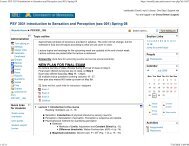
human observer. Is there a way to check? Suppose the signal and noise distributions look like: 

S1 S2 

σ n σ s 

X 

c 

possible criterion placement 

If we plot the hit rate vs. false alarm rate data on a graph, usually we get something that looks like: 


1 

Hit rate 

0 

0 1 

False alarm rate 

One can show that the area under this ROC curve is equal to the proportion correct in a two-alternative forced-choice 

experiment (Green and Swets). (Sometimes, sensitivity is operationally defined as this area. This provides a single summary 

number, even if the standard definition of d' is inappropriate, for example because the variances are not equal.) 

We return to our basic question: is there a way to spot whether our gaussian equal-variance assumptions are correct for 

human observers? 

If we take the same data and plot it in terms of Z-scores we get something like: 

Z(Hit rate) 

slope = σ n /σ s 

Z(False alarm rate) 

(µ s - µ n )/ σ s 

In fact, if the underlying distributions are Gaussian, the data should lie on a straight-line. If they both have equal variance, 

the slope of the line should be equal to one. This is because: 

Z ( hit rate ) 

X 

= 

Z ( false alarm rate ) 

− 

σ 

c s 

X 

= 

µ 

− 

σ 

c n 

n 

µ 

And if we solve for the criterion Xc, we obtain: 

s


σ 

n 

Z( hit rate ) = Z( false alarm rate ) − 

σ 

µ − µ 

σ 

s n 

(I've switched notation here, where s2 = µs, and s1 = µn). The main point of this plot is to see if the data tend to fall on a 

straight line with slope of one. If a straight line, this would support the Gaussian assumption. A slope = 1 supports the 

assumption of equal variance Gaussian distributions. 

In practice, there are several ways of obtaining an ROC curve in human psychophysical experiments. One can vary 

the criterion that an observer adopts by varying the proportion of times the signal is presented. As observers get used to the 

signal being presented, for example, 80% of the time, they become biased to assume the signal is present. One needs to 

block trials in groups of, say 400 trials per block. Where the signal and noise priors are fixed for a given block. 

One can also use a rating scale method in which the observer is asked to say how confident she/he was (e.g. 5 

definitely, 4 quite probable, 3 don't know for sure, 2, unlikely, 1 definitely not). Then we can bin the proportion of "5's" 

when the signal vs. noise was present to calculate hit and false alarm rates for that rating, do the same for the "4's", and so 

forth. The assumption is that an observer can maintain not just one stable criterion, but four---the observer has in effect 

divided up the decision variable domain into 5 regions. An advantage of the rating scale method is efficiency--relatively few 

trials are required to get an ROC curve. Further, in some experiments, ratings seem psychologically natural to make. But if 

there is any "noise" in the decision criterion itself, e.g. due to memory drift, or whatever, this will act to decrease the 

estimate of d' in both yes/no and rating methods. 

Usually rather than manipulating the criterion, we would rather do the experiment in such a way that it does not 

change. Is there a way to reduce the problem of a fluctuating criterion? 

The 2AFC (two-alternative forced-choice) method 

‡ Relating performance (proportion correct) to signal-to-noise ratio, d'. 

In psychophysics, the most common way to minimize the problem of a varying criterion is to use a two-alternative forcedchoice 

procedure (2AFC). In a 2AFC task the observer is presented on each trial a pair of stimuli. One stimulus has the 

signal (e.g. bright flash), and the other the noise (e.g. dim flash). The order, however, is randomized. So if they are presented 

temporally, the signal or the noise might come first, but the observer doesn't know which from trial to trial. In the 

spatial version, the signal could be on the left of the computer screen with the noise on the right, or vice versa. One can 

show that for 2AFC: 

d ' = - è!!!! 2 z Hproportion correctL 

(16) 

If you want to prove this for yourself, here are a couple of hints--actually, a lot of hints. Let us imagine we are giving the 

light discrimination task to the ideal observer. We have two possibilities for signal presentation: Either the signal is on the 

left and the noise on the right, or the signal is on the right and the noise on the left. There are two ways of being right. The 

observer could say "on the left" when the signal is on the left, or "on the right" when the signal is on the right. For example, 

for the light detection experiment, a reasonable guess is that all the ideal observer would have to do is to count the number 

of photons on the left side of the screen and count the number on the right too. If the number on the left is bigger than the 

number on the right, the observer should say that the signal was on the left. Thus, a 2AFC decision variable would be the 

difference between the left and right decision variables, where each of these is what we calculated for the yes/no 

experiment. 

r = rL - rR 

(17) 


For example, rL and rR for the SKE observer would be the dot products of the signal pattern template with observation 

image vectors on the left and right sides. 

So, the probabililty of being correct is: 

pc = p(r>0|signal on left) p(signal on left) + p(r


‡ Z-score. You used the inverse of a standard mathematical function called Erf[] to get Z from a measured P. 

z[p_] := Sqrt[2] InverseErf[1 - 2 p]; 

where Z(*) is the z-score for P c , the proportion correct. 

dprime[x_] := N[-Sqrt[2] z[x]] 

‡ Adaptive procedures for finding thresholds using 2AFC or yes/no. 

There have been a number of advances in the art of efficiently finding values of a signal which produce a certain percent 

correct in a psychophysical task such as 2AFC. For more on this, see the QUEST procedure of Watson and Pelli (1983) and 

the analyses of Treutwein (1993). 

Appendices 

Figure code 

Exercises 


References 

Applebaum, D. (1996). Probability and Information . Cambridge, UK: Cambridge University Press. 

Burgess, A. E., Wagner, R. F., Jennings, R. J., & Barlow, H. B. (1981). Efficiency of human visual signal discrimination. 

Science, 214, 93-94. 

Duda, R. O., & Hart, P. E. (1973). Pattern classification and scene analysis . New York.: John Wiley & Sons. 

Golden, R. (1988). A unified framework for connectionist systems. Biological Cybernetics, 59, 109-120. 

Green, D. M., & Swets, J. A. (1974). Signal Detection Theory and Psychophysics . Huntington, New York: Robert E. 

Krieger Publishing Company. 

Kersten, D. and P.W. Schrater (2000), Pattern Inference Theory: A Probabilistic Approach to Vision, in Perception and the 

Physical World, R. Mausfeld and D. Heyer, Editors. , John Wiley & Sons, Ltd.: Chichester. 

Kersten, D. (1984). Spatial summation in visual noise. Vision Research, 24,, 1977-1990. 

Kersten, D. (1999). High-level vision as statistical inference. In M. S. Gazzaniga (Ed.), The New Cognitive Neurosciences -- 

2nd Edition (pp. 353-363). Cambridge, MA: MIT Press. 

Knill, D. C., & Richards, W. (1996). Perception as Bayesian Inference. Cambridge: Cambridge University Press. 

Knill, D. C., Kersten, D., & Yuille, A. (1996). A Bayesian Formulation of Visual Perception. In K. D.C. & R. W. (Eds.), 

Perception as Bayesian Inference (pp. Chap. 0): Cambridge University Press. 

Ripley, B. D. (1996). Pattern Recognition and Neural Networks. Cambridge, UK: Cambridge University Press. 

Treutwein, B. (1993). Adaptive psychophysical procedures: A review. submitted to Vision Research, (email: 

bernhard@tango.imp.med.uni-muenchen.de) 

Van Trees, H. L. (1968). Detection, Estimation and Modulation Theory . New York: John Wiley and Sons. 

Watson, A. B., & Pelli, D. G. (1983). QUEST: A Bayesian adaptive psychometric method. 33, 113-120. 

Watson, A. B., Barlow, H. B., & Robson, J. G. (1983). What does the eye see best? Nature, 31,, 419-422. 

Yuille, A. L., & Bülthoff, H. H. (1996). Bayesian decision theory and psychophysics. In K. D.C. & R. W. (Eds.), Perception 

as Bayesian Inference. Cambridge, U.K.: Cambridge University Press. 

© 2000 Daniel Kersten, Computational Vision Lab, Department of Psychology, University of Minnesota. 

(http://vision.psych.umn.edu/www/kersten-lab/kersten-lab.html)

Computational Vision U. Minn. Psy 5036 Daniel Kersten Lecture 6

You also want an ePaper? Increase the reach of your titles

Delete template?

Save as template?