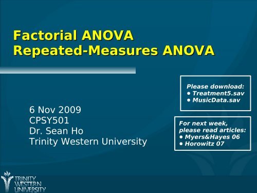
Factorial ANOVA Repeated-Measures ANOVA

Factorial ANOVA 

Repeated-Measures ANOVA 

6 Nov 2009 

CPSY501 

Dr. Sean Ho 

Trinity Western University 

Please download: 

● Treatment5.sav 

● MusicData.sav 

For next week, 

please read articles: 

● Myers&Hayes 06 

● Horowitz 07

Outline for Today 


● Running in SPSS and interpreting output 

● Main effects and interactions 

● Follow-up analysis: plots & simple effects 


● Assumptions: parametricity, sphericity 

● Follow-up analysis: post-hoc comparisons 

CPSY501: Factorial and RM ANOVA 

6 Nov 2009

Intro to Factorial ANOVA 

ANOVA with multiple “between-subjects” IVs 

Describe number of categories/groups per IV: 

● “5 x 4 x 4 design” means 3 IVs, with 

5 values (groups), 4 values, 4 values each 

Each cell is a combination of categories: 

● 5 x 4 x 4 = 80 cells 

● Each participant goes in exactly one cell, 

and is measured only once on the DV 

● Cells are assumed to be independent 

● “Balanced”: cell sizes all equal 


6 Nov 2009

Why Factorial ANOVA? 

Why not just do One-way on each IV? 

● IVs may have shared variance 

● Interaction effects (moderation)! 

Main effects: effect of just one IV (One-way) 

Two-way interaction: Effects of one IV change 

depending on value of another IV (moderator) 

3-way and higher interactions exist, too 

Higher-order effects supercede low-order ones: 

interpret the highest significant interaction 

Graphs may be needed to understand them 


6 Nov 2009




● Follow-up procedures 

● Interactions, main effects, & simple effects 

● Examples 


● Assumptions, sphericity 



6 Nov 2009

Factorial ANOVA in SPSS 

First check assumptions (see later slides) 

Analyze → GLM → Univariate 

● Enter all IVs together in “Fixed Factor(s)” 

● Model: “Full Factorial” (default) 

(checks for all main effects & interactions) 

● Options: Effect size & Homogeneity tests, 

Descriptives (and later, marginal means) 

Examine each effect in the model separately 

Treatment5.sav: IVs: Treatment Type, Gender 

● DV: just depression at outcome for now 


6 Nov 2009

Interpreting Output: Treatment5 

There were significant effects for treatment type, 

F (2, 21) = 21.14, p < .001, η 2 = .668, and gender, 

F (1, 21) = 14.69, p = .001, η 2 = .412, but 

no significant interaction, Tests of Between-Subjects F (2, 21) Effects = 0.15, 

p > .05, η 2 = .014 

Dependent Variable: depression levels at outcome of therapy 

Source 

Type III Sum 

of Squares df Mean Square F Sig. 

Partial Eta 

Squared 

Corrected Model 55.796(a) 5 11.159 11.431 .000 .731 

Intercept 317.400 1 317.400 325.141 .000 .939 

Gender 14.341 1 14.341 14.691 .001 .412 

Treatmnt 41.277 2 20.638 21.142 .000 .668 

Gender * Treatmnt .283 2 .142 .145 .866 .014 

Error 20.500 21 .976 

Total 383.000 27 

Corrected Total 

CPSY501: 76.296 Factorial and 26 RM ANOVA 

a R Squared = .731 (Adjusted R Squared = .667) 

6 Nov 2009






● Examples 





6 Nov 2009

Follow-up Analysis: Main effects 

If there are significant main effects: 

● Analyze → GLM → Univariate → Post-hoc 

● Post-hoc tests as in one-way ANOVA 

● SPSS does post-hoc for each IV separately 

(i.e., as if doing multiple one-way ANOVAs) 

Report means and SDs for each category of 

each significant IV (Options: Descriptives) 

Or report marginal means for “unique effects” 

(Options: Estimated Marginal Means) 

(more on this momentarily) 


6 Nov 2009

Post-hoc: Treatment5 

Post-hoc on main effect for Treatment Type: 

● Levene's is not significant, so can choose a 

post-hoc test that assumes equal variance: 

e.g., Tukey's HSD 

No post-hocs needed for Gender – why? 

Output on next slide: 

● The Wait List control group has significantly 

higher depression levels at post-treatment 

● (can graph means to visualize) 


6 Nov 2009

D e p e n d e n t V a ria: db ele 

p re s sio n le ve ls a t o u tc o m e o f th e ra p y 

M u ltip le C o m p a ris o n s 

T u k e y H S DC B T 

M e a n 

(I) T re a tm e n t T y p e(J) T re a tm e n t T y p eD iffe re n c(I-J) e S td. E rro r S ig. 

C B T 

9 5 %C o n fid e n ce In te rv a l 

U p p e r B o u n dL o w e r B o u n d 

C h u rc h-b a s e d 

s u p p o rt g ro u p -1 .1 2 .4 5 4 .0 5 5 -2 .2 7 .0 2 

C h u rc h-b a se d 

s u p p o rt g ro u p 

W L C o n tro l 

W L C o n tro l -3 .0 3(*) .4 6 9 .0 0 0 -4 .2 1 -1 .8 4 

C B T 1 .1 2 .4 5 4 .0 5 5 -.0 2 2 .2 7 


s u p p o rt g ro u p 

W L C o n tro l -1 .9 0(*) .4 8 0 .0 0 2 -3 .1 1 -.6 9 

C B T 3 .0 3(*) .4 6 9 .0 0 0 1 .8 4 4 .2 1 


s u p p o rt g ro u p 1 .9 0(*) .4 8 0 .0 0 2 .6 9 3 .1 1 

W L C o n tro l 

B a s e d o n o b se rve d m. 

e a n s 

* T h e m e a n d iffe re n c e is s ig n ific a n.0 t 5 ale t th vee 

. l 


6 Nov 2009

Estimated Marginal Means 

Estimate of group means in the population 

rather than the sample, accounting for 

effects of all other IVs and any covariates. 

Analyze → GLM → Univariate → Options: 

Move IVs and interactions to “Display means” 

● Select “Compare main effects” 

● Select multiple comparisons adjustment 

Can be used to obtain estimated means for: 

● (a) each group within an IV, and 

● (b) each cell/sub-group within an interaction 


6 Nov 2009

Actual vs. Estimated Means 

If instead we want to plot the 

actual sample group means, just use: 

Graph → Line → Multiple → Define: 

● Enter DV in Lines Represent menu, as 

“Other Statistic” 

● Enter IVs as “Category Axis” and 

“Define Lines By” 

Usually, the estimated marginal means are 

close to the actual sample means 


6 Nov 2009

Graphing Interactions 

For significant interactions: Graph the 

interaction to understand its effects: 

● Analyze → GLM → Univariate → Plots 

● SPSS plots estimated marginal means 

The IV with the most groups usually goes into 

“Horizontal axis” (if makes sense conceptually) 

For 3-way interactions, use “Separate plots”. 

More complex interactions require more work 


6 Nov 2009

Interactions Ex.: MusicData 

Dataset: MusicData.sav 

DV: Liking (scale) 

IV: Age (categorical: 0-40 vs. 40+) 

IV: Music (cat.: Fugazi, Abba, Barf Grooks) 

Run a 2x3 factorial ANOVA 

● Any significant interactions & main effects? 

● Plot the interaction of Age x Music 


6 Nov 2009


6 Nov 2009

Follow-up: Simple Effects 

If BOTH interaction and main effects are 

significant, report both but 

● Interpret the main effects primarily 

“in light of” the interaction 

How do we further understand effects? 

Simple effect: look at the effect of certain IVs, 

with the other IVs fixed at certain levels 

● e.g., do the old like “Barf Grooks” more than 

the young do? (fix Music = “Barf Grooks”) 

May need advanced SPSS syntax tools to do 


6 Nov 2009

Simple effects: MusicData 

Data → Split file → “Compare groups”: Music 

● Beware loss of power anytime we split data, 

due to small cell sizes 

Run an ANOVA for each group in Music: 

● GLM → Univariate: Liking vs. Age 

● Options: Effect size, Levene's tests, etc. 

Analogous to 3 t–tests for age: 

one t-test for each music group 


6 Nov 2009

Non-significant Interactions 

If the interaction is not significant, 

we might not have moderation. Either: 

● Leave it in the model (may have some minor 

influence, should be acknowledged), or 

● Remove it and re-run ANOVA 

(may improve the F-ratios) 

Analyze → GLM → Univariate → Model → Custom 

● Change Build Term to “Main effects” 

● Move all IVs into “Model”, but 

omit the non-significant interaction term 


6 Nov 2009

ANOVA: Parametricity 

Interval-level DV, categorical IVs 

Independent scores: look at study design 

Normal DV: run K-S & S-W tests 

Homogeneity of variances: 

● Levene’s tests for each IV 

● Really, need homogeneity across all cells 

Use the same strategies for 

(a) increasing robustness and 

(b) dealing with violations of assumptions 

as you would in one-way ANOVA 


6 Nov 2009

Assumptions: Practise 

Dataset: treatment5.sav 

DV: depression score at follow-up (scale) 

IV: Treatment (categorical: CBT vs. CSG vs. WL) 

IV: Age (scale, but treat as categorical) 

What assumptions are violated? 

For each violation, what should we do? 

After assessing the assumptions, run the 

Factorial ANOVA and interpret the results. 


6 Nov 2009






● Examples 





6 Nov 2009

TREATMENT 

RESEARCH 

DESIGN 

Cognitive- 

Behavioural 

Therapy 

Pre-Test Post-Test Follow-up 

Factorial 

ANOVA 

Church-Based 

Support Group 

Wait List 

control group 

Repeated 

Measures 

ANOVA 


6 Nov 2009

Between- vs. Within- Subjects 

Between-Subjects Factor/IV: 

Different sets of participants in each group 

● e.g., an experimental manipulation is done 

between different individuals 

● One-way and Factorial ANOVA 

Within-Subjects Factor/IV: The same set of 

participants contribute scores to each cell 

● e.g., the experimental manipulation is done 

within the same individuals 

● Repeated-Measures ANOVA 


6 Nov 2009

RM Example: Treatment5 

DV: Depressive symptoms 

● (healing = decrease in reported symptoms) 

IV1: Treatment group 

● CBT: Cognitive-behavioural therapy 

● CSG: Church-based support group 

● WL: Wait-list control 

IV2: Time (pre-, post-, follow-up) 

There are several research questions we could 

ask that fit different aspects of this data set 


6 Nov 2009

Treatment5: Research Qs 

Do treatment groups differ after treatment? 

● One-way ANOVA (only at post-treatment) 

Do people “get better” while they are waiting to 

start counselling (on the wait-list)? 

● RM ANOVA (only WL control, over time) 

Do people in the study get better over time? 

● RM ANOVA (all participants over time) 

Does active treatment (CBT, CBSG) decrease 

depressive symptoms over time more than WL? 

● Mixed-design ANOVA 

(Treatment effect over time) 


6 Nov 2009


One group of participants, experiencing all 

levels of the IV: each person is measured 

multiple times on the DV. 

● Scores are not independent of each other! 

RM is often used for: 

● (a) developmental change (over time) 

● (b) therapy / intervention (e.g., pre vs. post) 

● Also for other kinds of dependent scores 

(e.g., parent-child) 


6 Nov 2009

Why Use RM ANOVA? 

Advantages: 

● Improve power: cut background variability 

● Reduce MS-Error: same people in each cell 

● Smaller sample size required 

Disadvantages: 

● Assumption of sphericity is hard to attain 

● Individual variability is “ignored” 

rather than directly modelled: 

may reduce generalizability of results 

Use RM when you have within-subjects factors 


6 Nov 2009






● Examples 





6 Nov 2009

Assumptions of RM ANOVA 

Parametricity: (a) interval-level DV, 

(b) normal DV, (c) homogeneity of variances. 

● But not independence of scores! 

Sphericity: homogeneity of variances of 

pairwise differences between levels of the 

within-subjects factor 

● Test: if Mauchly’s W ≈ 1, we are okay 

● If the within-subjects factors has only 2 cells, 

then W=1, so no significance test is needed. 


6 Nov 2009

Treatment5: 3-level RM 

Analyze → GLM → Repeated Measures 

● “Within-Subject Factor Name”: Time 

● “Number of Levels”: 3, press “Add” 

Define: identify specific levels of the 

“within-subjects variable”: order matters! 

For now, don’t put in treatment groups yet 

(Look at overall pattern across all groups) 

Options: Effect size 

Plots: “Time” is usually the horizontal axis 

Look through the output for Time only! 


6 Nov 2009

Check Assumptions: Sphericity 

“The assumption of sphericity was violated, 

Mauchly’s W = .648, χ 2 (2, N = 30) = 12.16, p = .002.” 

If violated, use Epsilon (Greenhouse-Geisser) to 

adjust F-score (see later) 

Scored from 0 to 1, with 1 = perfect sphericity 

Measure: MEASURE_1 

Within Subjects Effect 

CHANGE 

Mauchly's W 

Mauchly's Test of Sphericity 

Approx. 

Chi-Square df Sig. 

Epsilon a 

Greenhous 

e-Geisser Huynh-Feldt Lower-bound 

.648 12.154 2 .002 .740 .770 .500 

Tests the null hypothesis that the error covariance matrix of the orthonormalized transformed dependent variables is 

proportional to an identity matrix. 

a. May be used to adjust the degrees of freedom for the averaged tests of significance. Corrected tests are displayed in the 

Tests of Within-Subjects Effects table. 


6 Nov 2009

If Sphericity Is Satisfied: 

Report F-ratio, df, p, and effect size from the line 

with Sphericity Assumed 

APA style: “F(2, 58) = 111.5, p < .001, η 2 = .794” 

If the omnibus ANOVA is significant, identify 

specific group differences using post hoc tests 


6 Nov 2009

If Sphericity Is Violated: 

F-ratio and ANOVA results may be distorted 

Consider multi-level modelling instead 

(but it requires much larger sample size), or 

Consider multivariate F-ratio results (MANOVA): 

● But it loses power compared to RM ANOVA 

● Need Greenhouse-Geisser epsilon ≤ .75 

● Need sample size ≥ 10 + (# “within” cells) 

● Report, e.g.: “Wilk’s λ = .157, 

F(2, 28) = 75.18, p < .001, η 2 = .843” 

(APA: Greek letters are not italicized) 


6 Nov 2009

Sphericity Violated: Adjust df 

Use Greenhouse-Geisser epsilon if ≤ .75: 

● If > .75, you may use the more optimistic 

Huynh-Feldt epsilon 

● Multiply df by epsilon and update F and p 

● This is given in the output tables 

If the adjusted F-ratio is significant, 

proceed to follow-up tests as needed 

Report: e.g., “Greenhouse-Geisser adjusted 

F(1.48, 42.9) = 111.51, p < .001, η 2 = .794” 


6 Nov 2009






● Examples 





6 Nov 2009

Follow-up analysis: post-hoc 

If the overall RM ANOVA is significant, explore 

differences between specific cells/times: 

● Analyze → GLM → Repeated Measures: 

Define → Options: 

● Estimated Marginal Means: 

move RM factor to “Display means for” 

● Select “Compare Main Effects”, use 

“Confidence interval adjustment”: 

Bonferroni 

Plot the effects over time: 

● Plots → IV in “Horizontal axis” → Add 

● Or try error bar plots 


6 Nov 2009

Post hoc comparisons, cont. 

Note: the Post-Hoc button applies only to 

between-subjects factors 

● Hence not applicable here: we only have 

one IV (Time) and it is within-subjects 

Interpret the output: 

● Bonferroni results show that the mean 

Pre-test scores are significantly higher than 

the mean Post-test & Follow-up scores 

● But the Post-test & Follow-up scores are not 

significantly different 

● (see “Pairwise Comparisons”, “Estimates”) 


6 Nov 2009

Practise: Field-Looks_Charis.sav 

Dataset: “Looks & Charisma” (from Field text) 

How does “attractiveness” change over time? 

How does “charisma” change over time? 

Combine both IVs in a factorial RM analysis 

(using both IVs) 

Attending to sphericity issues, interpret the 

results 

Conduct follow-up tests to see which kinds of 

people are evaluated more (and less) positively 


6 Nov 2009

Factorial ANOVA Repeated-Measures ANOVA

You also want an ePaper? Increase the reach of your titles

Delete template?

Save as template?